Disk ICs

Here are my notes at setting up a disk made of self-gravitating particles. For now there is no background potential, but I will add that in later.

I’ll be following the disk model from Hernquist 1993. There are probably more recent models that we could use if this isn’t good enough.

Positions

The positions are selected from sampling the density profile:

\[\rho(R,z) = \dfrac{M_d}{4 \pi h^2 z_0} \exp(-R/h) {\rm sech}^2 \left(\dfrac{z}{z_0} \right)\]

Radius

The probability that a particle is within radius \(R\) is given by

\[P(<R) = \dfrac{\int_{-\infty}^\infty \int_0^R \rho R' {\rm d}R' dz'}{\int_0^\infty \int_0^\infty \rho R' {\rm d}R' {\rm d}z'}\]

This simplifies nicely for the given disk model to \(P(<R) = 1-\exp(-R/h)\).

Therefore, I selected a random number, \(A\) between 0 and 1 for each particle, and solved for the radius, \(R = -h \ln (1-A)\).

Height

The probability it will be at height \(z\), given that it is at radius \(R\), is:

\[P(<z) = \dfrac{2 \pi \int_{-\infty}^z \rho {\rm d}z'}{2 \pi \int_{-\infty}^\infty \rho {\rm d}z'}\]

For our model, \(P(<z) = (\tanh(z/z_0)+1)/2\), so given a random number \(A\) between 0 and 1 for each particle, the height is, \(z = z_0 {\rm arctanh} (2A -1)\).

Cartesian positions

To convert the radial position, \(R\), to cartesian coordinates \(x\), \(y\), for each particle I randomly selected an angle \(\theta\) between \(0\) and \(2 \pi\), and then solved \(x=R \cos(\theta)\), \(y = R \sin(\theta)\).

Velocities

I did my best to follow Hernquist here, though there were a couple points I wasn’t entirely clear on. For the most part, I assumed all the particles were located at \(z=0\), so these approximations are probably only valid for a very thin disk.

I also found these notes helpful.

Tangential velocity

The velocity in \(v_z\) was drawn from a Gaussian with a dispersion of \(\sqrt{\bar{v_z^2}}\).

The dispersion was calculated for an isothermal sheet,

\(\bar{v_z^2} = \pi G \Sigma(R) z_0\),

I assumed that \(\Sigma(R)\) is the total surface density, \(\Sigma(R) = \int \rho {\rm d}z\); for our model:

\[\Sigma(R) = \dfrac{M_d}{2 \pi h^2} \exp(-R/h)\]

Radial velocity

The radial velocity was also calculated by drawing from a Gaussian. In this case, they set the velocity dispersion to:

\[\bar{v_R^2} \approx Q \sigma_{R, {\rm crit}}(R_{\rm ref}) \exp(-R/h)\]

Where \(\sigma_{R, {\rm crit}}(R) = \dfrac{3.36 G \Sigma (R)}{\kappa(R)}\) is the critical radial dispersion for axisymmetric stability. This is evaluated at \(R_{\rm ref}\), which is a reference point in the disk corresponding to \(Q\), the Toomre parameter specified at that radius. \(R_{\rm ref}\) is typically \(2\)-\(3h\).

\[\kappa^2 = \dfrac{3}{R}\dfrac{\partial \Phi}{\partial R } + \dfrac{\partial^2 \Phi}{\partial R^2}\]

is the epicyclic frequency (note that the potential here should be from ALL contributions). In the case we are only considering the disk, but later we can add in the potential of the halo.

For an axisymmetric disk, the potential should follow:

\[\dfrac{\partial^2 \Phi}{\partial z^2} + \dfrac{1}{R}\dfrac{\partial}{\partial R} \left( R \dfrac{\partial \Phi}{\partial R}\right)= 4 \pi G \rho\]

There are methods in Binney and Tremaine for how to approximate this, or I could solve the PDE numerically.

Instead, I am going to assume the disk is infinitely thin, and use equation 2.191 in Binney and Tremaine (first edition):

\[\Phi(R,\phi) = - G \int_0^\infty {\rm d}R' R' \int_0^{2 \pi} {\rm d} \phi'\dfrac{\Sigma(R',\phi')}{\sqrt{R'^2 + R^2 - 2 R R' \cos(\phi'-\phi)}}\]

Since the system is axisymmetric, I will just set \(\phi\) to zero, and then solve the equation numerically.

Azimuthal Velocity

The azimuthal velocity, \(v_{\phi}\), has two components: the streaming and random component.

First, the streaming component, \(\bar{v_\phi}\), can be approximated as:

\[\bar{v_\phi}^2 - v_c^2 = \bar{v_R^2} \left(1 - \dfrac{\kappa^2}{4 \Omega ^2} - 2\dfrac{R}{h} \right)\]

\(\Omega\) is the angular frequency. This can be solved from the potential, from the equation \(R \Omega^2 = \dfrac{ {\rm d} \phi} { {\rm d} R}\).

\(v_c\) is the circular velocity \(\sqrt{GM(<R)/R}\). The enclosed mass can be determined from, \(M(<R) = 2 \pi \int_0^R \Sigma(R')R' dR'\), and therefore the circular velocity is:

\[v_c^2 = \dfrac{G M_d}{ R} (1 - (R/h +1) \exp(-R/h))\]

Secondly, the random component is selected from a Gaussian with dispersion \(\sqrt{\sigma_\phi^2}\), where:

\(\sigma_\phi^2 = \bar{v_R^2} \dfrac{\kappa^2}{4 \Omega^2}\).

Finally, \(v_{\phi}\) is assigned as by adding the random component to the streaming component, \(\bar{v_\phi}\).

Note that sometimes these approximations break down at small radii. If this is a problem, we can “soften” \(\bar{v_R^2}\) (see Equation 2.29 in Hernquist 1993). For now I’m ignoring this potential problem.

You can see that changing the Toomre parameter will change the radial dispersion, which in term will change the azimuthal velocity, and control the rotation of the disk.

Cartesian Velocities

Note that the radial velocity is \(v_r=\dot{r}\) and the azimuthal velocity is \(v_{\phi}=r\dot{\phi}\). Take derivatives of \(x(r,\phi)\) and \(y(r,\phi)\) to find:

\[v_x = v_{r} \cos(\theta) - v_{\phi} \sin(\theta)\] \[v_y = v_{r} \sin(\theta) + v_{\phi} \cos(\theta)\]

Stability of Isolated Disk

To test the stability of the disk, I evolved \(10^5\) disk particles in isolation in Gadget-2 (no background potential), with the parameters \(Md = 1\), \(h = 1\), \(z_0 = 0.2\), \(G = 1\), \(Q = 1.5\), \(R_{\rm ref}= 8.5/3.5\) (these can be scaled to appropriate units). I set the softening length to \(0.1\).

Here is how it looks:

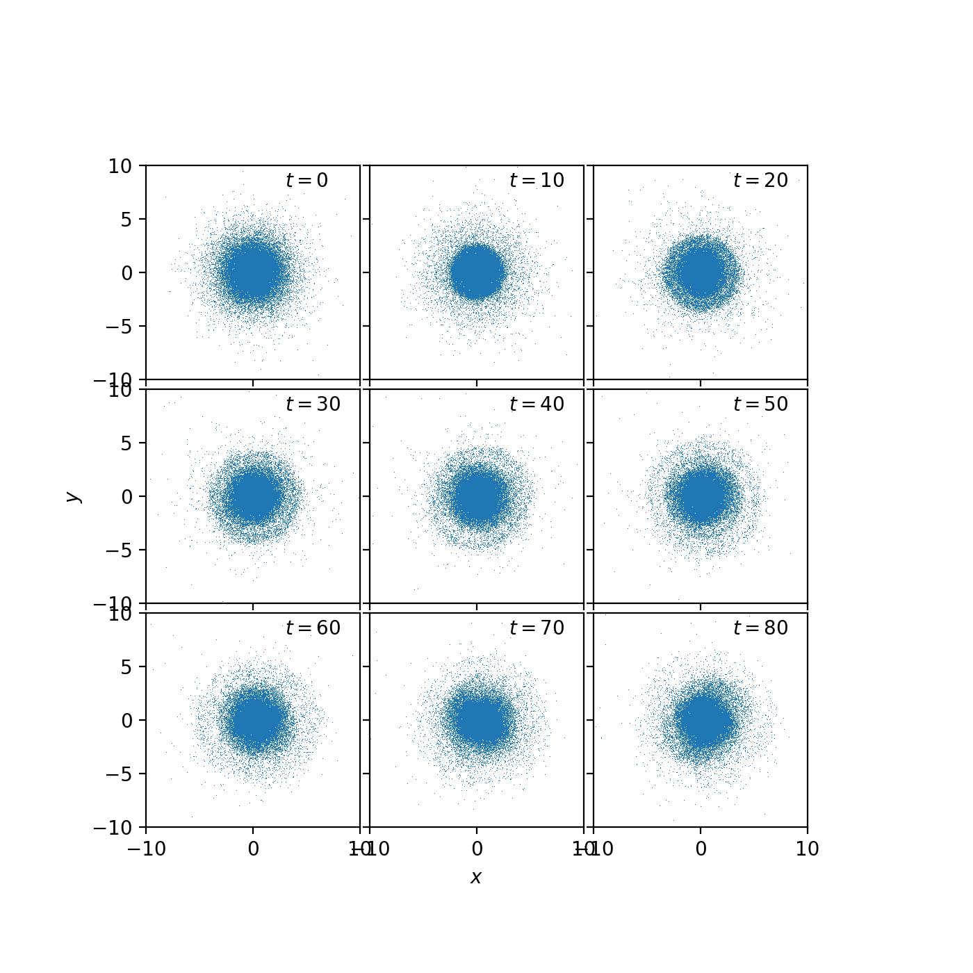
This seems roughly stable. I want to go over my calculations and code to make sure I don’t have any errors, and plot the density profiles and see if they look stable. I also need to calculate the softening more carefully.

Adding in Halo Potential

Next I’m going to add in the halo potential, which will change the assigned velocities. Then I’ll add in the potential for the gas in the disk.

---

Disk ICs with Halo Potential »