JWST Pipeline

Here are my notes on the JWST Calibration Pipeline.

General Workflow

Get data: The “raw” data can either be downloaded from MAST, or simulated with MIRAGE.
Inspect data: “You can use JWST data analysis tools to inspect the highest level of science calibration pipeline products produced for a given instrument mode’s data to determine whether they are satisfactory for your science.”
Calibration pipeline: You can run the “science calibration pipeline, if desired, to reprocess the data. Standard science calibration pipeline processing should produce publication-quality data products for most cases.”

I have a MIRAGE image working. I want to examine this a little more to see what is reasonable. Caitlin said to run it through the calibration pipeline as “that’s where some problems start to come up that is present in real data as well as simulations, like the astrometry issue, background subtraction, 1/f noise, etc”.

My Questions:

Is the pipeline continuously being updated? I.e. is it worth my time to got through all the issues if they will be fixed soon?
What would people want from the DREaM simulated images? Should I provide a calibrated image, or would others (e.g. the imaging team) want to run those things themselves?

I guess it is worth it for me to roughly go through this process, to get an idea of how the pipeline works, and whether my images look reasonable! I can decide later whether it is worthwhile for me to polish everything up to get science-ready images from the DREaM catalog. Note that I think I need to go through the pipeline to add the exposures together.

Starting File

In the previous post I made a test image in Mirage. This is what the *_uncal.fits file looks like (opened in DS9).

My Questions:

Is this really what the raw data looks like?
I assume I want to run this for every pointing, and then add the images together. Do they get added together before or after the calibration pipeline? I think this is answered by the pipeline process!

Calibration Pipeline

In this post, I’m going to focus on going through the steps to run the pipeline on the image shown above.

Install Calibration Pipeline

Installation instructions are here

I simply used pip install jwst. I also need CRDS reference files, but I already set this up (see previous post).

Science Calibration Pipeline Stages

The pipeline has three steps:

Stage 1: Apply detector-level corrections to the raw data for individual exposures and produce count rate (slope) images from the “ramps” of non-destructive readouts

Stage 2: Apply physical corrections (e.g., slit loss) and calibrations (e.g., absolute fluxes and wavelengths) to individual exposures

Stage 3: Combine the fully calibrated data from multiple exposures

I’m going to go through these steps using these notes

Stage 1

Stage 1 takes the _uncal.fit file and creates _rate.fits and _rateints.fits files.

I first tried to run everything together:

# The entire calwebb_detector1 pipeline
from jwst.pipeline import calwebb_detector1

# Individual steps that make up calwebb_detector1
from jwst.dq_init import DQInitStep
from jwst.saturation import SaturationStep
from jwst.superbias import SuperBiasStep
from jwst.ipc import IPCStep
from jwst.refpix import RefPixStep
from jwst.linearity import LinearityStep
from jwst.persistence import PersistenceStep
from jwst.dark_current import DarkCurrentStep
from jwst.jump import JumpStep
from jwst.ramp_fitting import RampFitStep
from jwst import datamodels

uncal_file = glob(simdata_output_dir+'/*_uncal.fits')[0]

detector1 = calwebb_detector1.Detector1Pipeline()
detector1.output_dir = pipeline_output_dir
detector1.save_results = True
detector1.persistence.input_trapsfilled=persist_file

However, this seemed to hang, and I wasn’t sure where, so I ran the steps separately to trouble shoot

# 1. Data Quality Initialization
dq_init_step = DQInitStep()
dq_init_step.output_dir = pipeline_output_dir
dq_init_step.save_results = True
dq_init = dq_init_step.run(uncal_file)

# 2. Saturation Flagging
saturation_step = SaturationStep()
saturation_step.output_dir = pipeline_output_dir
saturation_step.save_results = True
saturation = saturation_step.run(dq_init)

# 3. Superbias Subtraction
superbias_step = SuperBiasStep()
superbias_step.output_dir = pipeline_output_dir
superbias_step.save_results = True
superbias = superbias_step.run(saturation)

# 4. Reference Pixel Subtraction Step
refpix_step = RefPixStep()
refpix_step.output_dir = pipeline_output_dir
refpix_step.save_results = True
refpix = refpix_step.run(superbias)

# 5. Linearity Correction
linearity_step = LinearityStep()
linearity_step.output_dir = pipeline_output_dir
linearity_step.save_results = True
linearity = linearity_step.run(refpix)

# 6. Persistence Correction

persist_step = PersistenceStep()
persist_step.output_dir = pipeline_output_dir
persist_step.save_results = True
persist = persist_step.run(linearity)

# 7. Dark Current Subtraction
dark_step = DarkCurrentStep()
dark_step.output_dir = pipeline_output_dir
dark_step.save_results = True
dark = dark_step.run(persist)

# 8. Cosmic Ray Flagging
jump_step = JumpStep()
jump_step.output_dir = pipeline_output_dir
jump_step.save_results = True
jump = jump_step.run(dark)

# 9. Ramp_Fitting
ramp_fit_step = RampFitStep()
ramp_fit_step.output_dir = pipeline_output_dir
ramp_fit_step.save_results = True
ramp_fit = ramp_fit_step.run(jump)

List of problems I ran into:

saturation_step: “ValueError: too many values to unpack (expected 2)”. Micaela said it was probably an incompatibility with stcal and jwst. Updating jwst fixed my problem :) (I’m now running stcal v1.1.0 and jwst v1.6.2)
dark step: “cannot reshape array of size 517993664 into shape (187,2048,2048)””. This seemed to be a problem with the file in the crds_cache, “crds_cache/references/jwst/nircam/jwst_nircam_dark_0341.fits”, so I deleted it. When I reran the dark step it re-downloaded this file. This was very slow for some reason today, and took about 2 hours for the 6GB file!

Once I fixed these problems, I could run the whole Step 1.

My Questions:

Should I get a traps-filled file for persistence step?
What are all the options for running step 1? Should I alter any of the defaults?

Stage 2

“The Stage 2 pipeline applies instrumental corrections and calibrations to the slope images output from Stage 1. This includes background subtraction, the creation of a full World Coordinate System (WCS) for the data, application of the flat field, and flux calibration. In most cases the final output is an image in units of surface brightness. Whereas the input files had suffixes of _rate.fits, the output files have suffixes of _cal.fits. The Stage 2 pipeline can be called on a single fits file, or a collection of fits files. When calling on multiple files, the input is a json-formatted file called an “association” file that lists each of the fits files to be processed.”

I ran this on the one _rate.fits file from Stage 1. This didn’t throw any errors.

My Questions:

What are all the options for running step 2? Should I alter any of the defaults?

Stage 3

“The Stage 3 pipeline takes one or more calibrated slope images (_cal.fits files) and combines them into a final mosaic image. It then creates a source catalog from this mosaic. Several steps are performed in order to prepare the data for the mosaic creation. There are three final outputs. The first is updated copies of the input files (_i2d.fits). These updated files contain a consistent WCS, such that they overlap correctly. The second output is a final mosaic image (_segm.fits) created by drizzling the input images onto a distortion-free grid. And the final output is a source catalog (_cat.ecsv) wth basic photometry, created from the final mosaic image.”

Again, I just ran this on the one pointing, and it seemed to work fine.

My Questions:

What are all the options for running step 3? Should I alter any of the defaults?

Final thoughts

Here is the image from MIRAGE (top left), after Stage 1 (top right), after Stage 2 (bottom left) and after Stage 3 (bottom right)

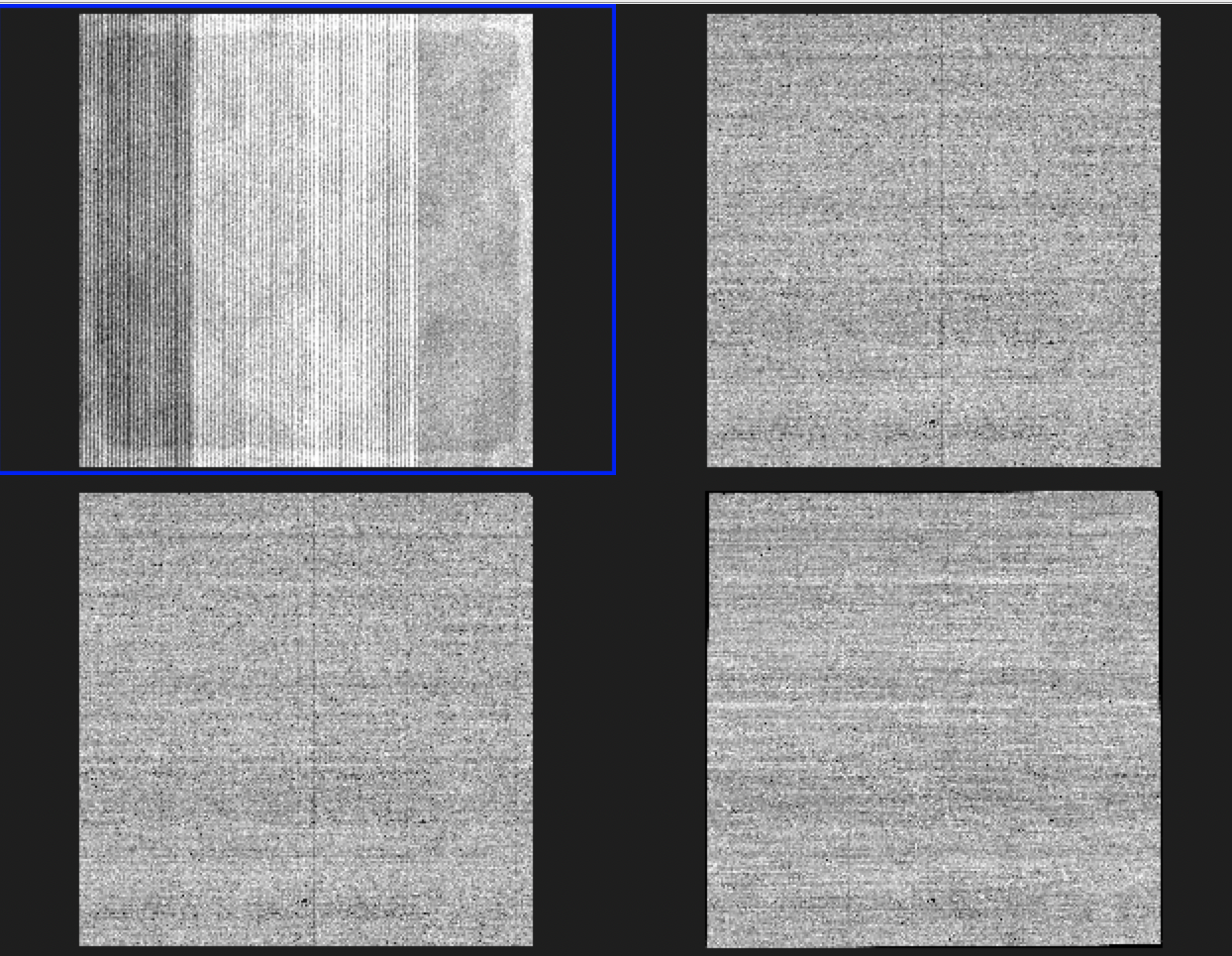
I obviously still need to sort out a lot of details, but this seems like it is sort of working.

Main next steps:

Add my catalog
Get a pipeline working so that I can run this on multiple pointings
Go through the MIRAGE generation to make sure I am selecting all the parameters carefully
Go through JWST pipeline to make sure I’m selecting all the parameters carefully

« Mirage

Add Catalog to Mirage »