Nicole Drakos
Research Blog
Welcome to my Research Blog.
This is mostly meant to document what I am working on for myself, and to communicate with my colleagues. It is likely filled with errors!
This project is maintained by ndrakos
LF Environmental Dependance
One main advantage of COSMOS-Web is that it will be able to look at the bright end of the LF in different environments for high-redshift galaxies.
For this project I want to explore different predictions for how the UVLF should vary in different environments for different underlying models, and see whether COSMOS-Web can constrain this.
In this post, I’m going to go through environmental measurements, and preliminary results with the baseline DREaM Catalog.
Environmental Measures
There is a nice summary of different environmental measures used in the literature in Muldrew et al. 2012. They review 20 different measurements of environment, but “most methods fall into two broad groups: those that use nearest neighbours to probe the underlying density field and those that use fixed apertures.” Their conclusion is that “When considering environment, there are two regimes: the ‘local environment’ internal to a halo best measured with nearest neighbour and ‘large-scale environment’ external to a halo best measured with apertures.”
Measuring Environment in my Catalog
Clearly environmental measures will depend on how many/which galaxies I include. For now I will do a cut in MUV at -18. I think this is roughly the limit COSMOS-Web will have at high redshifts. I will still measure environment for all the galaxies, but only consider neighbours brighter than -18. For some methods I will only consider galaxies in the same redshift bin; e.g., if the galaxy is at redshift 6.7, it will be considered z~7, since it is in the bin [6.5,7.5]. I will then use all galaxies in that redshift bin when calculating the local density.
Below, I list the density measurements I will consider to start with. While these methods aren’t the best representation of observational methods, they should give an idea if there is an environmental dependance, and whether this dependancy depends on how the environment is measured. I may in the future modify/add to these measurements.
1) 3rd nearest neighbour in 3D
The “density” can be approximated by finding the distance to the \(n\)th nearest neighbour, \(r_n\), and then calculating:
\[\Sigma = \dfrac{n}{4/3 \pi r_n^3}\]I will use \(n=3\), and the comoving distance.
2) 3rd projected nearest neighbour
This is similar to above, but with
\[\sigma = \dfrac{n}{\pi r_n^2}\]I will again use \(n=3\). Now I’m going to take the position in RA and Dec though.
3) 3rd projected nearest neighbour (in redshift bin)
Same as (2) but only considering galaxies in the same redshift bin.
4) In a fixed aperture
In this method, the aperture is held fixed, and the density inside the aperture is calculated as
\[\delta \dfrac{N_g-\bar{N_g}}{\bar{N_g}}\]where \(N_g\) is the number of galaxies inside the aperature, and \(\bar{N_g}\) is the mean number that would be expected if galaxies were distributed randomly (i.e. it is the total number of galaxies divided by the area multiplied by the aperture size). I chose the aperture to have a radius of 0.001 degrees.
This clearly could have some weird effects since if the galaxies are randomly distributed in the volume of the survey, they will not be evenly distributed in the projected area. This should be mostly mitigated in the next method.
5) In a fixed aperture (in redshift bin)
Same as (4), but only considering galaxies in the same redshift bin
Results - UV Luminosity Functions
Here are some results, where I have split the galaxies in 5 quintiles and plotted their luminosity functions (multiplied by a factor of 5, so I could compare to the total luminosity function in black). 1st quintile galaxies are are the least dense environments, while the 5th quintile galaxies are in the most dense environments.
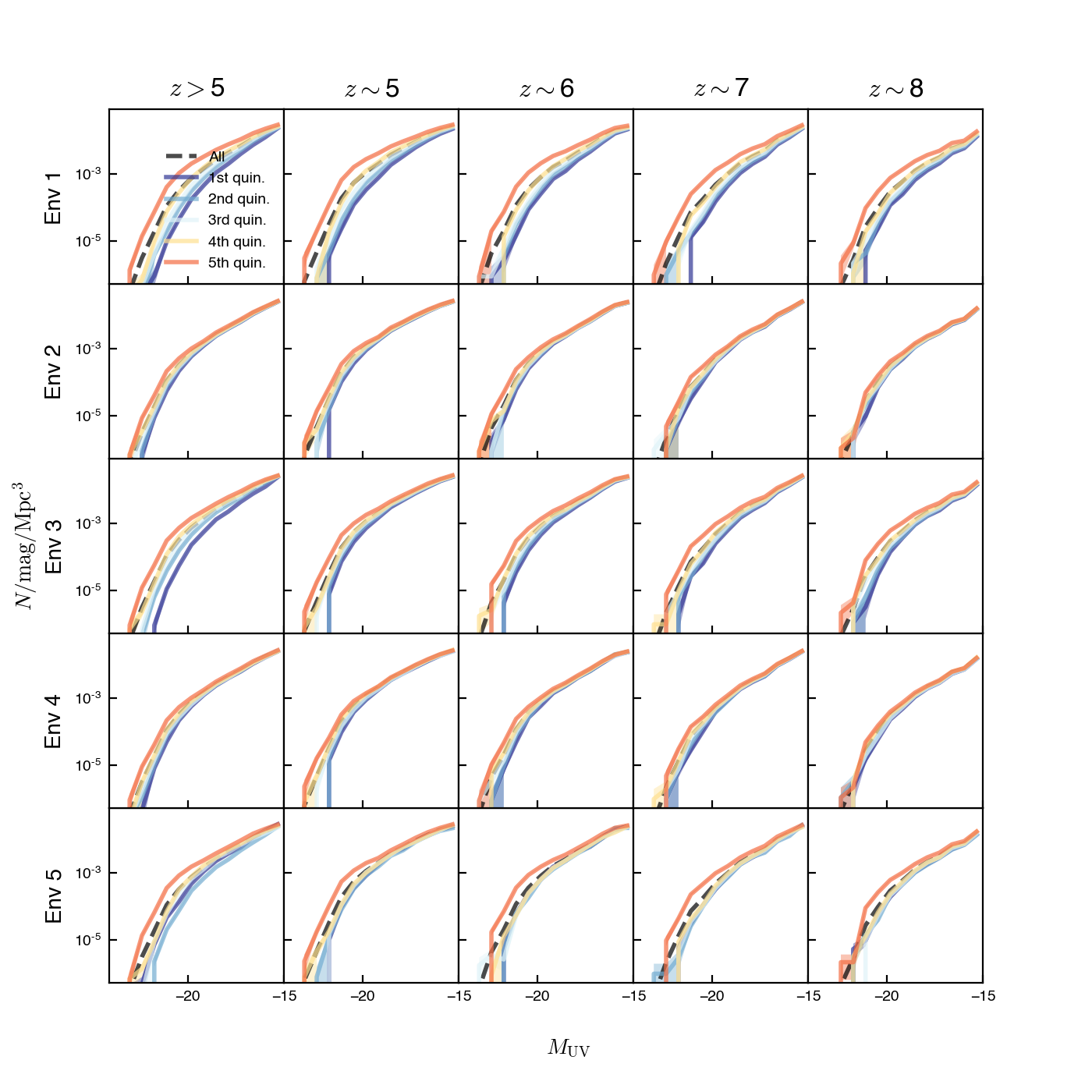
Comments on plot:
- Brighter galaxies tend to be in denser regions.
- Env 1 and Env 3 are probably the best measurements, but all the measurements qualitatively agree.
- Note Env 4 measurement has a lot of objects with an Env measurement of -1, so the sorting is not the clearest (this could probably be improved by increasing the aperture size)
- Once I look at determining the difference between different models, I also want to plot the luminosity function in different JWST bands.
Varying the Underlying Model
Right now the DREaM model effectively goes from halo mass -> galaxy mass -> M_UV, where the first is from abundance matching, and the second is from the Mass-M_UV relation in Williams et al. 2018.
- What assumptions are built into this?
- How does the underlying reionization model change the LF? I.e., do galaxies in ionized regions have different LFs than galaxies in non-ionized regions?
- What other physical processes/modelling assumptions affect the environmental dependance?
This will require a bit of lit review and thought from me, and I’ll probably make a post about it in the future.