Changes to SED Method

In previous posts, I detailed a method for assigning SED parameters, but had trouble reproducing the expected trends in \(M_{UV}\) and \(\beta\). (See e.g., this post.)

New Method

Now I am assigning \(M_{UV}\) and \(\beta\) directly, and then fitting the age and dust (which are the least well constrained parameters).

Specifically, I assigned \(M_{UV}\) and \(\beta\) directly from the mean relations (no scatter), and the SFR, metallicity and gas ionization were assigned as before.

For the fitting procedure I am using scipy.optimize.brute. This uses a grid search method, and then a local solver to “polish” the solution. I then used these best-fit dust and age values to calculate the UV properties of the galaxies.

I ran this for a subsample of 16000 randomly selected galaxies from the \(512^3\) simulation, and got the following:

Now I am able to reproduce the trends. Even though the assigned UV properties did not have any scatter from the relation, there is some scatter in the above relation because the parameters were not fit perfectly.

Timing Considerations

This took ~1.5 hr to run on a subsample of 16000 galaxies using 400 cores.

The \(2048^3\) simulation will have approximately \(10^8\) galaxies (calculated by integrating the redshift-dependant HMF over the survey volume):

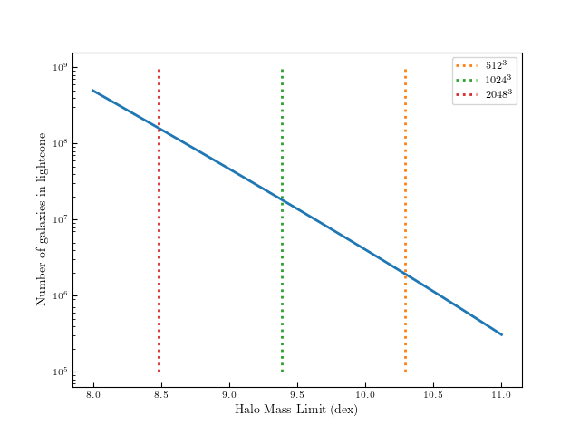
Therefore the current method is not feasible to run on the \(2048^3\) simulation.

I profiled the code, and the slow part is that every galaxy ends up calling FSPS ~500 times.

New New Method

The new plan is to create a grid of potential spectra. For now, I will call this the “base catalog” (need a better name though). Each point on this (non-uniform) grid will be assigned 7 parameters: redshift, mass, age, dust attenuation, \(\tau\), metallicity and gas ionization. FSPS will be used to generate a spectra at this point, which can then be used to calculate the SFR, \(M_{UV}\) and \(\beta\).

Once this “base catalog” is created, I will create a k-d tree of the catalog in 7 parameter space (redshift, mass, metallicity, gas ionization, SFR, \(M_{UV}\) and \(\beta\)).

Then, to assign spectra for each galaxy in the real catalog (each with an associated redshift and mass)

1. I will “propose” values for metallicity, gas ionization, SFR, \(M_{UV}\) and \(\beta\) (same as before)
2. I will find the 10 nearest neighbours in the k-d tree
3. I interpolate to get the the 5 input params to FSPS (age, dust, tau, metallicity, gas ionization) (weighted by the distance to each neighbour)
4. Then, given these interpolated values, I will call FSPS (now only 1 FSPS call per galaxy) to get SFR, \(M_{UV}\) and \(\beta\) (these will not be identical to the input values, but should be close)

Based on some very rough calculations, I should be able to generate \(10^8\) spectra in approximately a day. Step 4 will then be very doable for the \(2048^3\) catalog.

I have tested this on a couple of points, and it seems to work well (just using my 16000 galaxy sample to generate the k-d tree). The generation of the k-d tree, and the measurement of the nearest neighbours took a negligible amount of time with this small problem.

The next steps:

1. Test this on a larger number of galaxies to make sure I am recovering the input scaling relations
2. Make a new “base catalog” (I need to decide how many points, how to sample the 7D space)

---

« Galaxy Sizes Part III

SED Pipeline »