Check IC Power Spectrum

I decided to write my own simple IC code, and add neutrinos to that. Here are my notes on checking the IC Power Spectrum of the dark matter particles, to make sure my IC code is working correctly.

Input Power Spectrum

As I said before, I’m using camb to generate the powerspectrum. Here is how it is made:

params = camb.CAMBparams()
params.set_cosmology(H0=H0, ombh2=Omega_b/h**2, omch2=(Omega_m-Omega_b)/h**2)
params.InitPower.set_params(ns=nspec)
params.set_matter_power(redshifts=[z_start,0])
PK = camb.get_matter_power_interpolator(params,var1='delta_tot',var2='delta_tot')

From what I could tell, CAMB doesn’t allow you to specify the sigma_8 value, but does allow you to specify the amplitude (which is set to some default value). My (not very elegant, but quick) fix is:

#set normalization of power spectrum from sigma_8
results = camb.get_results(params)
kh, z, pk = results.get_matter_power_spectrum()
A = sigma_8**2/results.get_sigma8_0()**2
params.InitPower.As *= A
PK = camb.get_matter_power_interpolator(params,var1='delta_tot',var2='delta_tot')

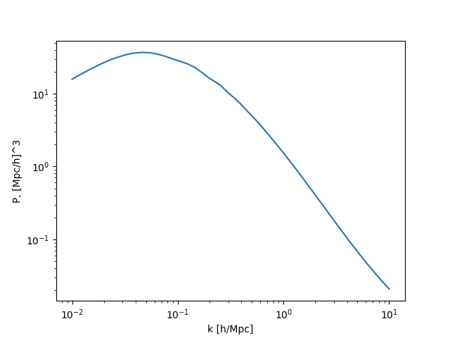
Here is the input spectrum:

Spectrum from Particles

I want to compare the input spectrum to the particle matter spectrum, and make sure they match

Download and Install Pylians

I decided to use Pylians to calculate the particle power spectrum.

I cloned github repository, and then used

cd library
python setup.py install

To test it was working, I tried python Tests/import_libraries.py. At first this said pyfftw wasn’t installed, but after I pip installed it was fine.

Plotting Particle Power Spectrum

Here’s how to plot power in pylians (documentation):

import MAS_library as MASL
import Pk_library as PKL
MAS     = 'CIC'  #mass-assigment scheme, use cloud-in-cell
verbose = False
nthreads=4

pos = np.array([x, y, z], dtype=np.float32).T
delta = np.zeros((N,N,N))
MASL.MA(pos, delta, boxlength, MAS, verbose=verbose)
delta /= np.mean(delta);  delta -= 1.0; delta = np.array(delta, dtype=np.float32)
PK_p= PKL.Pk(delta, boxlength, 0, MAS, nthreads, verbose)
k_p = PK_p.k3D
P_p = PK_p.Pk
plt.loglog(k_p, P_p)

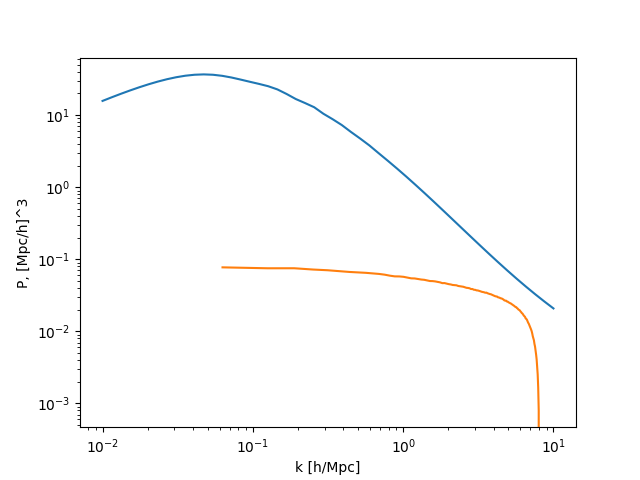
This is what I find:

Clearly these don’t match.

Trouble Shooting

Check initial density field

The initial density field is found by

1. make a random gaussian field \(\mu\), with mean 0 and variance 1
2. take FFT of \(\mu\)
3. Multiple \(\tilde\mu\) by \(\sqrt{P}\)
4. Inverse FFT

Here is my code:

density = random.randn(N,N,N) #gaussian field
density = np.fft.fftn(density) #fourier space
ka = 2*np.pi*fft.fftfreq(N, d=boxlength/N)
kx,ky,kz =np.meshgrid(ka,ka,ka)
k = np.sqrt(kx**2 + ky**2 + kz**2)
P = PK.P(z_start,k)
density = np.sqrt(P)*density
density_real =np.real(np.fft.ifftn(density)) #back to real space

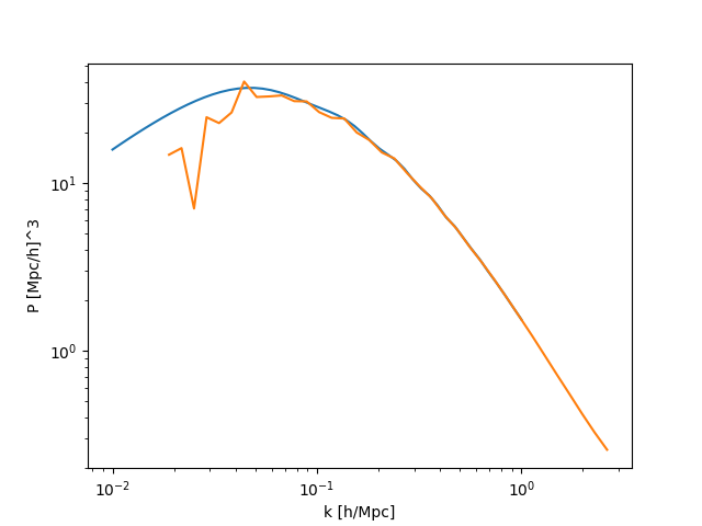
The density does seem to be real, which is reassuring. The overdensity should be between -1 and infinity. This actually goes from roughly -1.4 to 1.2. However, less than 1e-6 particles are below -1, so this is actually pretty good too. Here is the distribution of densities at the grid points:

When I check the power of this, compared to the initial density, I get:

PK_p= PKL.Pk(np.array(density_real, dtype=np.float32), boxlength, 0, 'None', nthreads, verbose)
k_p = PK_p.k1D
P_p = PK_p.Pk1D
plt.loglog(k_p, P_p)

This looks very close to the power spectrum I was getting for the particles so maybe something is going wrong here at this stage, OR I am plotting the power spectrum wrong.

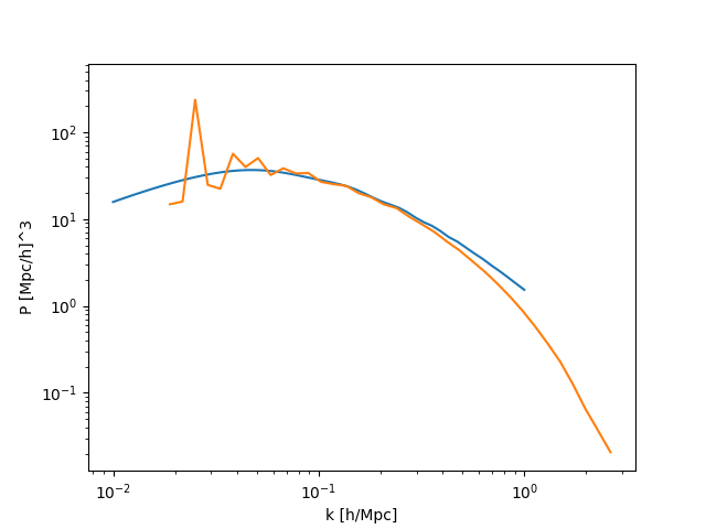
Here is my own calculation of the power spectrum:

fourier_amplitudes = np.abs(density)**2
fourier_amplitudes = fourier_amplitudes.flatten()
kbins = np.logspace(-2, 1,50)
kvals = 0.5 * (kbins[1:] + kbins[:-1])
Abins, _, _ = stats.binned_statistic(k.flatten(), fourier_amplitudes, statistic = "mean", bins = kbins)
P = Abins/N**3
plt.loglog(kvals, P)

which gives:

This looks right, so I guess I am misusing the PKL power spectrum library. I’m going to assume the density assignment is correct.

Check Particle Assignment

With this method of calculating the power spectrum, I can find the power of the particles as follows:

MAS = 'CIC'
pos = np.array([x, y, z], dtype=np.float32).T
delta = np.zeros((N,N,N),  dtype=np.float32)
MASL.MA(pos, delta, boxlength, MAS, verbose=verbose)
delta /= np.mean(delta);  delta -= 1.0; delta = np.array(delta)

delta_f = np.fft.fftn(delta)
fourier_amplitudes = np.abs(delta_f)**2
fourier_amplitudes = fourier_amplitudes.flatten()
kbins = np.logspace(-2, 1,50)
kvals = 0.5 * (kbins[1:] + kbins[:-1])
Abins, _, _ = stats.binned_statistic(k.flatten(), fourier_amplitudes, statistic = "mean", bins = kbins)
plt.loglog(kvals, Abins/N**3)

I find:

This looks much better, but doesn’t match on small scales. This could simply be that I didn’t correct for the cloud-in-cell (CIC) algorithm used to get the density field. I’m going to leave this for now, and move on. The positions look roughly right

Here is the CIC correction (see eq 27 in this paper):

delta_f = np.fft.fftn(delta)
if MAS=='NGP':
    p=1
elif MAS=='CIC':
    p=2
else:
    p=0
correct_x = (np.sin(kx * boxlength/(2*N)) / (kx * boxlength/(2*N))  )**(-p)
correct_y = (np.sin(kx * boxlength/(2*N)) / (kx * boxlength/(2*N))  )**(-p)
correct_z = (np.sin(kx * boxlength/(2*N)) / (kx * boxlength/(2*N))  )**(-p)
correct_x[np.isnan(correct_x)] = 1; correct_y[np.isnan(correct_y)] = 1; correct_z[np.isnan(correct_z)] = 1
correct = correct_x*correct_y*correct_z
fourier_amplitudes = np.abs(delta_f*correct)**2
fourier_amplitudes = fourier_amplitudes.flatten()
kbins = np.logspace(-2, 1,50)
kvals = 0.5 * (kbins[1:] + kbins[:-1])
Abins, _, _ = stats.binned_statistic(k.flatten(), fourier_amplitudes, statistic = "mean", bins = kbins)
plt.loglog(kvals, Abins/N**3)

I get:

This looks good! So I’m going to conclude that the particle position assignment is probably correct.

---

« Writing my own IC Code

Testing ICs in Gadget »