Reionization Shell Model Part II

I am planning to calculate the reionized region around each galaxy in the DREaM catalog using a simple shell model, following Magg et al. 2018..

This is a continuation from a previous post, Part I.

Thinking more about star formation histories

In the previous post, we showed how the rate of ionizing photons changed over time for some example galaxies:

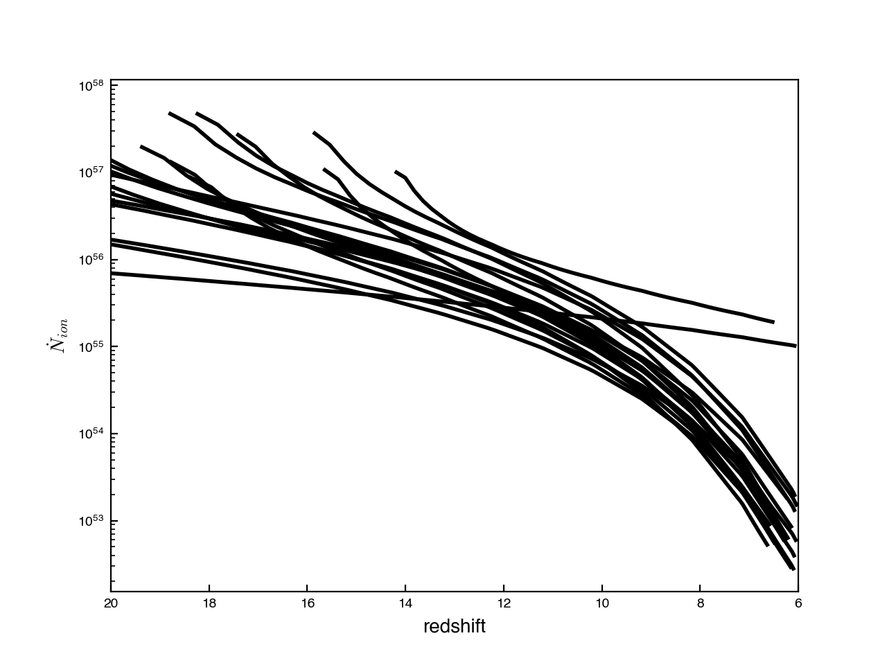
I can’t find any plots of this value to check the numbers against, but hoping I want to think a little bit about whether these trends make sense! The galaxies follow a delayed-tau model for the star-formation history (\(\psi \propto t e^{-t/\tau}\)). Here is an example pulled from the internet:

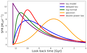
Every galaxy has two parameters to define this relation; one, \(\tau\), controls the “delay” term, and the second, \(t_{\rm start}\) controls when star formation starts. We will also use \(t_{\rm age}\) to define the age of the universe corresponding to the redshift of the galaxy. For delayed-tau models, we expect there to be a raid rise in the star formation rate, and then an exponential decline. The location of the peak of star-formation is at \(t=\tau\). If \(t_{\rm start}>\tau\), then the SFR is initially declining, and if \(t_{\rm start}<\tau\), the SFR is initially rising. Similarly, if \(t_{\rm age}>\tau\) then the SFR is currently declining, and if \(t_{\rm age}<\tau\), the SFH is currently rising.

Here is the distribution of redshifts:

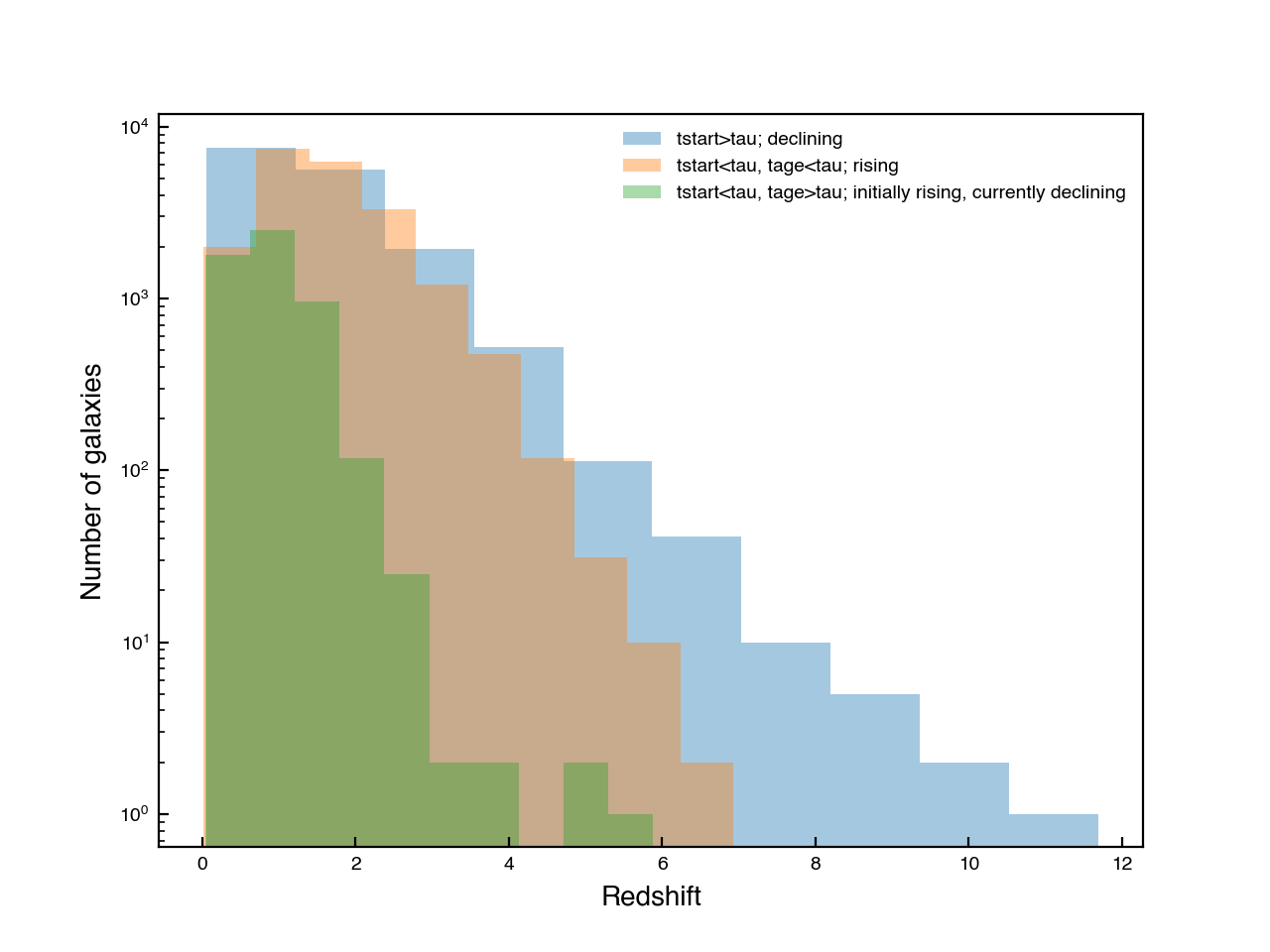
It seems that all the high redshift (\(z>7\)) galaxies have declining SFHs. As stated in the DREaM paper, one of the motivations for using the delayed-tau model was that high-redshift galaxies have rising SFHs (Finlator et al. 2011). However, with it seems our model favoured a solution where galaxies have declining SFRs at the highest redshifts. This explains why \(N_{\rm dot}\) decreased with time in each of the examples I plotted above. The physical scenario here could be that there is some early starburst, and then declining star formation rations.

I’m not too worried that this will effect the findings of Drakos+2022, since regular tau-models are often used in the literature. However, this might be a problem for our approach to modeling reionization bubbles, as outlined in Part I. For now, I will proceed with the calculations, using these SFHs, but if we get unphysical answers, it would be worth revisiting this!

Calculate the volume around individual galaxies

As outlined in the previous post, we expect the volume around each galaxy to be

\[V(t) = f_{\rm esc}\dfrac{e^{- n C \alpha t}}{n} \int e^{ n C \alpha t} \dot{N}_{\rm ion} dt\]

(Note that I have multiplied \(\dot{N}_{\rm ion}\) by \(f_{\rm esc}\); here I assume \(f_{\rm esc}\)=0.2 for all galaxies )

Looking at one galaxy, and assuming an initial condition of \(V(t_{\rm start}=0)\), I find:

These numbers seem too big to me. I expected that maybe by redshift 6 they would be ~1-10 Mpc for a single galaxy.

Next steps

1. Dig into the literature, and see what the expected volumes should be
2. Double check the derivation of this equation, and make sure the values I’m using make sense. Should any be time dependent?
3. Once I think this makes sense, write code to do this for all galaxies
4. Plot the reionized regions, see if they agree with radiative transfer simulation findings. (i.e., is the percentage of ionized regions reasonable?)

---

« Reionization Shell Model

Reionization Shell Model Part III »