Nicole Drakos
Research Blog
Welcome to my Research Blog.
This is mostly meant to document what I am working on for myself, and to communicate with my colleagues. It is likely filled with errors!
This project is maintained by ndrakos
2PCF of Mock Galaxies
In a previous post, I plotted the 2PCF for the galaxy catalog. There were some slight issues, which I am addressing here.
The Random Catalog
When comparing the distribution to that of a random catalog you need to make sure of two things (1) that you have the same sky coverage and (2) that the smoothed redshift distribution is the same.
The survey is a pyramid of height \(d_{\rm max}\) and length/width of \(d_{\rm max} \sin \theta\), where \(\theta\) is the survey volume (see this post).
Previously, I had distributed the galaxies uniformly in comoving space; therefore, I need to fix this to make sure I have the correct redshift distribution.
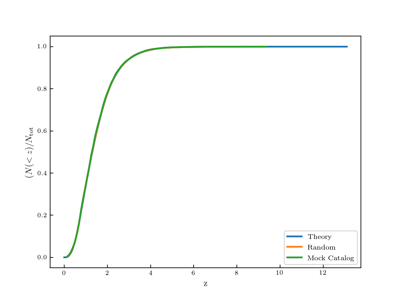
Given a SMF \(\phi\), you can calculate the number of galaxies in mass range \([M_1,M_2]\) and within a comoving distance \(d\) as:
\[N(<d) =\int_0^{V(d)} \int_{M_1}^{M_2} \phi(M,z(d)) \rm{d}M {\rm d}V\]given that a volume element is \({\rm V} = d^2 \sin^{2}(\theta) {\rm d}d\):
\[N(<d) = \sin^2(\theta) \int_0^d d^2 \int_{M_1}^{M_2} \phi(M,z(d)) dM {\rm d}d\]I checked this by plotting this theoretical \(N(<z)\) (calculated using the theoretical SMF), compared to the random sample I created and then comparing to the mock galaxy data (within a given mass range). They all agree very well:
Overall, the method for creating a mock galaxy is:
(1) pick a random number \({\rm rand}\) between \(0\) and \(1\), and then solve for \(N(<d)/N(<d_{\rm max})={\rm rand}\) to get the comoving distance, \(d\).
(2) generate two more random numbers and then solve for \(y = d \sin(\theta) ({\rm rand}-0.5)\) and \(z = d \sin(\theta) ({\rm rand}-0.5)\)
(3) Convert these to RA, DEC and distance as in this post
Methods
Same as before, I used corrfunc and chose \(\pi_{\rm max} = 20 {\rm Mpc}/h\)… This is generally chosen to minimize effects of redshift space distortions, but maximize signal to noise.
The error bars were determined by bootstrapping the data—in every bin, i resampled (with replacement) the data 200 times, and then found the mean and standard deviation in each bin.
Results
Here I am showing the results for galaxies in the mass range [10,10.5] \(M_{\odot}/h^2\)
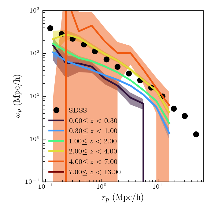
There appears to be a discrepancy between the SDSS data (from Yang et al. 2012) and the low redshift data. Additionally, I don’t know if I believe the redshift evolution that the plot shows.
Assuming this is correct, and that all the galaxies in this mass range should be detected, this demonstrates how well we will be able to measure the evolution of the galaxy correlation function in the UDF survey, though this will depend on the exact mass and redshift bins.
Compare to snapshots
I also compared to clustering measurements directly from the simulation (this requires running abundance matching on the individual snapshots). Calculating the clustering signal uses a different routine in corrfunc and doesn’t require the creation of a random catalog.
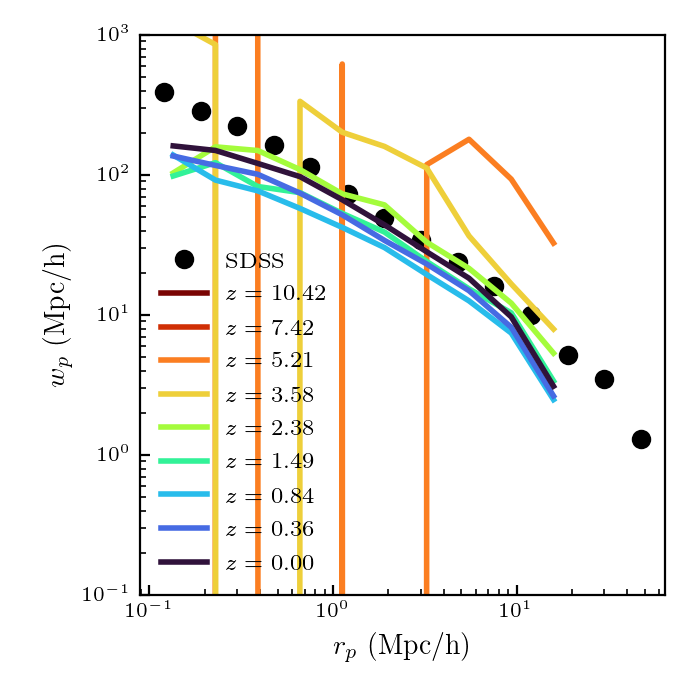
This agrees more with the SDSS data, and doesn’t show the same redshift evolution. I am not sure why this is.