Nicole Drakos
Research Blog
Welcome to my Research Blog.
This is mostly meant to document what I am working on for myself, and to communicate with my colleagues. It is likely filled with errors!
This project is maintained by ndrakos
Galaxy Clustering
In this post I will go over calculating the galaxy clustering signal, measured as the projected two-point correlation function (2PCF).
Two-Point Correlation Function
The 2PCF, \(\xi(r)\), is defined as the excess probability of finding galaxies separated by \(r\) (in units \(h^{-1}\, \rm{ Mpc}\)) compared to if the galaxies were distributed uniformly.
There are two main ways to measure this. The first method is by taking the inverse Fourier transfer of the power spectrum. The second method is to construct a random distribution of points (with the same sky coverage and smoothed redshift distribution), and then compare this to the galaxy distribution. There are several estimators of \(\xi(r)\) using this second method, the most common being the Landy-Szalay estimator.
(Brant has some code to calculate the power spectrum and Landy-Szalay 2PCF here and here, respectively.)
Projected Two-Point Correlation Function
To compare to observations, it is more convenient to define the projected 2PCF:
\[\omega_{\theta}(r_{p})= \int_{-\infty}^{\infty} \xi (r_p,\pi) \mathrm{d} \pi \approx 2 \int_{0}^{\pi_{max}} \xi (r_p, \pi) \mathrm{d} \pi\]where \(r_p\) and \(\pi\) are projected separation and the separation along the line-of-sight, respectively. The upper limit \(\pi_{\rm max}\) needs to be chosen carefully, and depends on the underlying survey (see van den Bosch et al. 2013 on discussion regarding this).
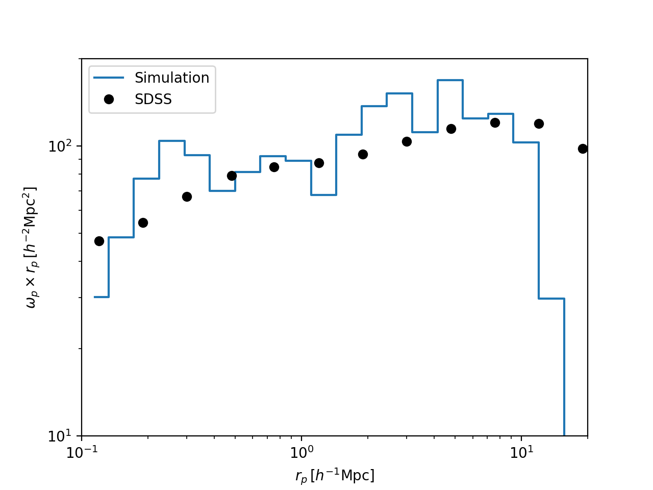
Results
I will perform SHAM on the sample simulation as outlined in this post. For now I am neglecting scatter in the abundance matching procedure.
I am going to use the package CORRFUNC to measure the projected correlation function. The value for \(\pi_{\rm max}\) should be set to \(40 h^{-1} \, {\rm Mpc}\) to be comparable to the SDSS data (following Campbell et al. 2018); my sample simulation does not have a large enough volume for this, so I am using \(20 h^{-1} \, {\rm Mpc}\), and then multiplying the correlation function by two (I think this works?). I am using CORRFUNC’s theory routine, which takes in cartesian coordinates and assumes the plane-parallel approximation—this should be okay under the assumption of a distant observer. Another option would be to calculate RA, DEC and redshifts for each galaxy, and use the mocks routine.
The projected 2PCF measured from SDSS DR7 can be found in Table 5 of Yang et al. 2012. Note that their masses are in units \(\log_{10}(1/M_{\rm sol} h^{-2})\). Therefore, I add \(\log_{10}h\) to my AHF masses before calculating the clustering.
Here are my results in the mass bin 10 to 10.5: