Nicole Drakos
Research Blog
Welcome to my Research Blog.
This is mostly meant to document what I am working on for myself, and to communicate with my colleagues. It is likely filled with errors!
This project is maintained by ndrakos
Two Component System
Peter said he was interested in doing his Lamat project on tidally stripped halos. I would like him to look a bit into how multi-component systems are stripped in energy space, but I am not sure how hard this will be to set up. Here I am going to test whether I can get the ICs work (I will then update my code online that makes ICs, and he could use that to set-up the simulations).
The Model
I need to think more about what is a realistic model to use. I am most interested in dwarf galaxies that have a dark matter and stellar component. Potentially this could be extended later to include a disk as well (Widrow et al. 2005 is probably one of the most useful references for this).
For now I am going to simply use two Hernquist models, as these are a simpler model (nice expressions for their denisty, mass and potential, and they don’t have a divergent mass profile):
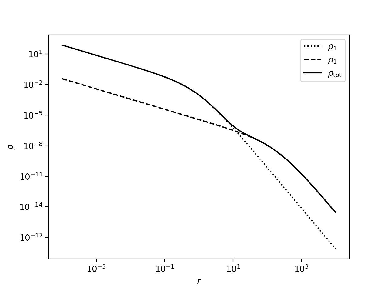
\[\rho = \dfrac{M_{\rm tot}a}{2\pi r (r+a)^3}\]I’ve used the parameters \(a_1=1\), \(a_2=200\), \(M_{\rm tot}=1\) and \(M_2=20 \,M_1\); note that the simulation can be scaled, so these are in arbitrary units, with \(G=1\). For the actual project, I’ll give a bit more thought into the best models/parameters to use.
Here is how this two-component model looks:
Assigning Particle Positions and Velocities
I have pretty detailed notes on created isolated ICs here.
Given that there are \(N_1\) particles in component 1, and \(N_2\) particles component 2, I wish to assign positions and velocities to each particle so that they remain stable. The density profile, mass profile and potential are additive (\(\rho= \rho_1+ \rho_2\), \(M = M_1+ M_2\), \(\Phi = \Phi_1 + \Phi_2\)). However, the difficulty with the two-component system is that the potential of each component affects the other, so the density profiles interact in complicated ways.
To generate the ICs, first, the positions are selected from the mass profile. This step is unchanged, and I can select positions for each component individually.
Given the position for each particle (and therefore the potential),the energies are selected from the distribution function. If I break up the distribution function into two, each part is given by:
\[f_i(\mathcal{E})=\dfrac{1}{\sqrt{8}\pi^2}\left[ \int_{r_{\mathcal{E}}}^\infty \dfrac{1}{\sqrt{\mathcal{E}- \Psi}}\dfrac{d^2 \rho_i}{d \Psi^2} \dfrac{GM}{r^2} dr \right]\]here, the relative potential \(\Psi\equiv-\Phi\) is from the total system, as are \(M\) and \(\rho\); it is only the one term \(\rho_i\) that differs between the two profiles. The energies can be selected from the distribution function for each component.
Once the position and energy are known, the velocity is \(v=\sqrt{2(\mathcal{E}-\Psi)}\).
Run in Isolation
I’ve generated the 2-component Hernquist system with \(10^5\) particles, and evolved it in isolation for \(t=500\) (simulation units). To get an idea of how long this is, I’ve drawn two vertical lines corresponding to the radius at which the time is equal to the relaxation timescale (dashed black line), and one corresponding to the radius at which the time is equal to the evaporation timescale (dotted black line):
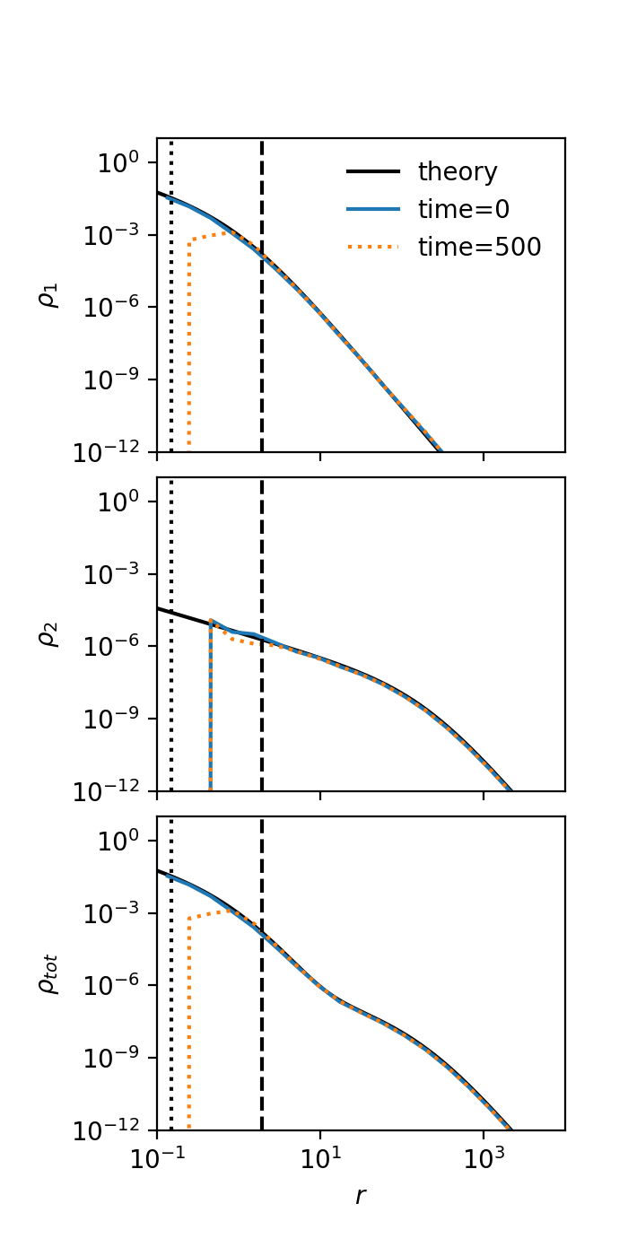
The system is stable outside the relaxation lengthscale, and I think it would be closer to the evaporation line if there were more particles (note that where the blue curve sharply drops in the second panel corresponds to the radius where the mass in component 2 is equal to the mass of one particle).
This seems to be working, so I will go ahead and assign this project.