Nicole Drakos
Research Blog
Welcome to my Research Blog.
This is mostly meant to document what I am working on for myself, and to communicate with my colleagues. It is likely filled with errors!
This project is maintained by ndrakos
Calculating Bound Mass
In a paper that is currently under revision, I determined the self-bound particles in a subhalo by iteratively removing any particles with a negative energy. This requires calculating the potential of all the particles in the subhalo. I had been assuming the remnant was spherically symmetric (which halo finders such as AHF assume as well), as this greatly reduces the computation time, but the reviewer raised concerns over how this might affect the results. These are some of my tests to see how the spherical approximation compares to calculating the full potential.
Potential Calculations
Spherical Approximation
For a spherically symmetric system, you can treat the mass of each particle \(i\) as being distributed over a shell of radius \(r_i\), and the potential at particle \(i\) becomes (see Drakos et al. 2019):
\[P_i \approx -Gm \left( \dfrac{N(<r_i)}{r_i} + \sum_{j=1,\\ r_j>r_i}^N \dfrac{1}{r_j} \right)\]Since this calculation involves distances \(r_i\) from the centre of the subhalo, it is much faster than calculating the distances between every pair of particles, \(r_{ij}\).
Full Potential
It is not feasible to calculate the full potential directly. As pointed out by the reviewer, in van den Bosch et al. 2018, they used the Barnes & Hut algorithm. However, I am going to calculate the potential energy as described in Bett et al. 2010:
\[P_i = \left(\dfrac{N-1}{N_{\rm sel}-1}\right) \left(\dfrac{-Gm}{\epsilon}\right) \sum_{j=1,\\ j \neq i}^{N_{\rm sel}} -W(r_{ij}/\epsilon)\]Here, \(N_{\rm sel}\) is the number of randomly selected particles used to approximate the entire distribution (each of these particles can be considered to have a mass \(m N/N_{\rm sel}\)). \(W\) is the smoothing kernel used for force calculations in GADGET-2:
\[W(x) = \begin{cases} \dfrac{16}{3}x^2 - \frac{48}{5}x^4 + \frac{32}{5} x^5 - \frac{14}{5}, & 0 \leq x \leq \frac{1}{2}\\ \frac{1}{15x} + \frac{32}{3}x^2 - 16 x^2 +\frac{48}{5}x^4\\ -\frac{32}{15}x^5 - \frac{16}{5}, & \frac{1}{2} \leq x \leq 1\\ -\frac{1}{x}, & x \geq 1 \,\,\, . \end{cases}\]As in Drakos et al. 2019, I will use \(N_{\rm sel}= 5000\) particles.
Results
I tested a few of the results for the Fast and Slow Simulations (described in the paper):
Mass loss curves:

Density profiles (taken at third apocentric passage):

Shape calculation:
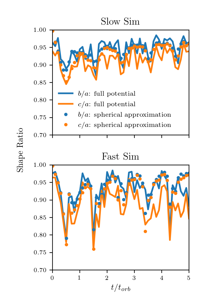
Conclusions
Even though there is quite a bit of noise associated with the method I used to calculate the full potential (this could be improved by repeating the method with another randomly selected subset of particles, and averaging the results), the two methods agree very well.