Nicole Drakos
Research Blog
Welcome to my Research Blog.
This is mostly meant to document what I am working on for myself, and to communicate with my colleagues. It is likely filled with errors!
This project is maintained by ndrakos
Adding Scatter
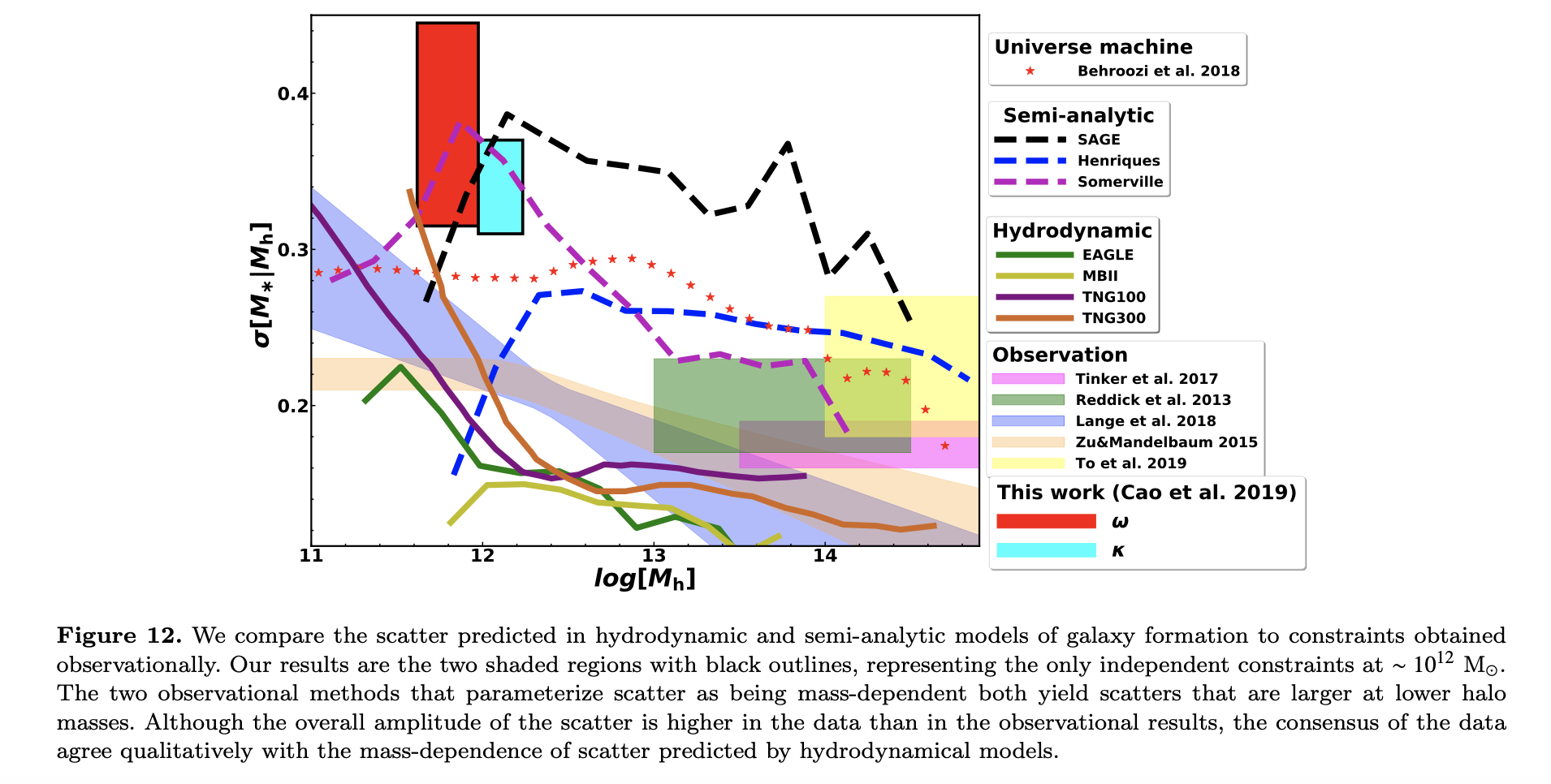
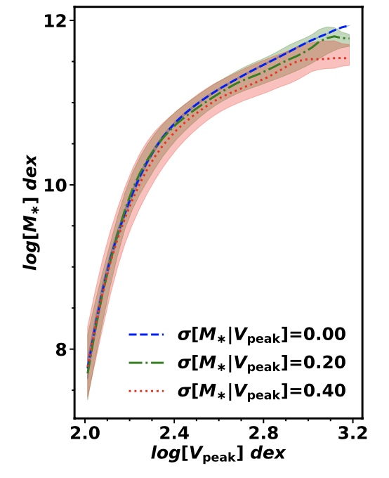
While basic subhalo abundance matching (SHAM) has no free parameters, it is common to introduce scatter in the stellar mass–halo mass (SM–HM) relation. For now I am setting a constant scatter of \(\sigma(M_* \mid v_{\rm peak}) \approx 0.2\) dex, which is common in in the literature. While there is some evidence that this scatter does not depend on halo mass (e.g. Yang et al 2009 + more recent references), it is not well constrained observationally for low mass halos. New constraints on the scatter at low masses can be found in Cao et al. 2019, and their summary plot on SM–HM scatter is is shown below:
Method 1: Deconvolution
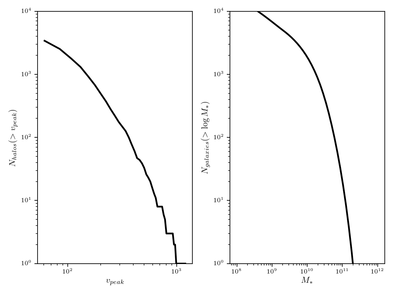
If including scatter, the stellar mass function (SMF) used in SHAM should be the intrinsic SMF, \(\phi_{\rm int}\), not the observed SMF, \(\phi_{\rm obs}\).
It is common to use the deconvolution method based on Behroozi et al. 2010 to determine the intrinsic SMF. As described in Reddick et al. 2013, this method can be described as follows:
(1) Estimate that \(\phi_{\rm int} = \phi_{\rm obs}\)
(2) Perform SHAM, as described here, using \(\phi = \phi_{\rm int}\)
(3) Add the scatter; we assume there is log normal scatter (e.g. draw a random number from a gaussian distribution with standard deviation of \(\sigma\), and add this to \(\log M_*\))
(4) Calculate the new SMF, \(\phi_{\rm scat}\); if we have the right intrinsic SMF, this should be equivalent to the observed SMF
(5) Re-estimate the new \(\phi_{\rm int}\) based on difference between the scattered SMF \(\phi_{\rm scat}\) and the observed SMF \(\phi_{\rm obs}\)
(6) Repeat steps 2-5 until \(\phi_{\rm int}\) converges
There are some difficulties in implementing this method; first of all it is not clear what is the best method to re-estimate \(\phi_{\rm int}\) in step (5), especially for bins with few halos. Also, the deconvolution is sensitive to the end points of the \(\phi_{\rm obs}\) and \(\phi_{\rm scat}\) (this typically requires extrapolation beyond these points). There is code available here to perform SHAM using this method of adding scatter. However, I am going to use the method detailed below.
Method 2: Add Scatter to Halo Property
Recently, Cao et al. 2019 suggested that a more operationally convenient method is to directly add scatter to the halo property before performing the abundance matching step. This requires finding the relationship between the given scatter in stellar mass, \(M_*\), and our chosen halo mass proxy, \(v_{\rm peak}\).
Create Look-up Table
(1) Vary \(\sigma(\log v_{\rm peak})\) from 0 to 0.5 linearly, using 500 points
(2) For each \(\sigma(\log v_{\rm peak})\), add scatter to \(v_{\rm peaks}\) (drawing from log-normal distribution)
(3) Perform SHAM
(4) From the output stellar masses, measure \(\sigma[\log M_*\mid \log v_{\rm peak}]\) as a function of (the un-scattered) \(v_{\rm peak}\)
Abundance Matching with Scatter
(5) For the given scatter \(\sigma[\log M_* \mid \log v_{\rm peak}]\) (which we choose to be 0.2) find the corresponding scatter \(\sigma(\log v_{\rm peak})\)
(6) Perform steps (2)-(3) with the appropriate \(\sigma(\log v_{\rm peak})\)
Things to Think About
Does this method for scatter create any biases/have any assumptions?
Does adding log-normal scatter in \(v_{\rm peak}\) result in log-normal scatter in \(M_*\)? (can check this)
Results – Troubleshooting
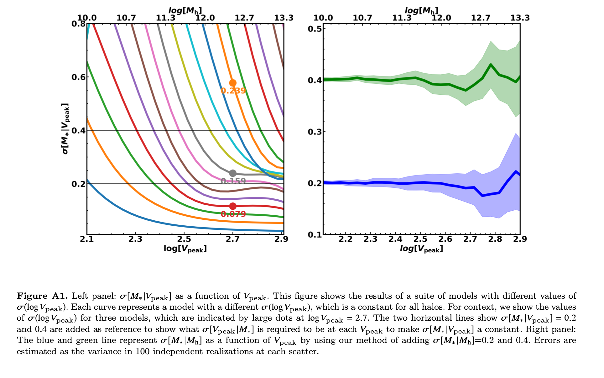
I am trying to reproduce the following plot from Cao et al. 2019
However my plot looks like this:
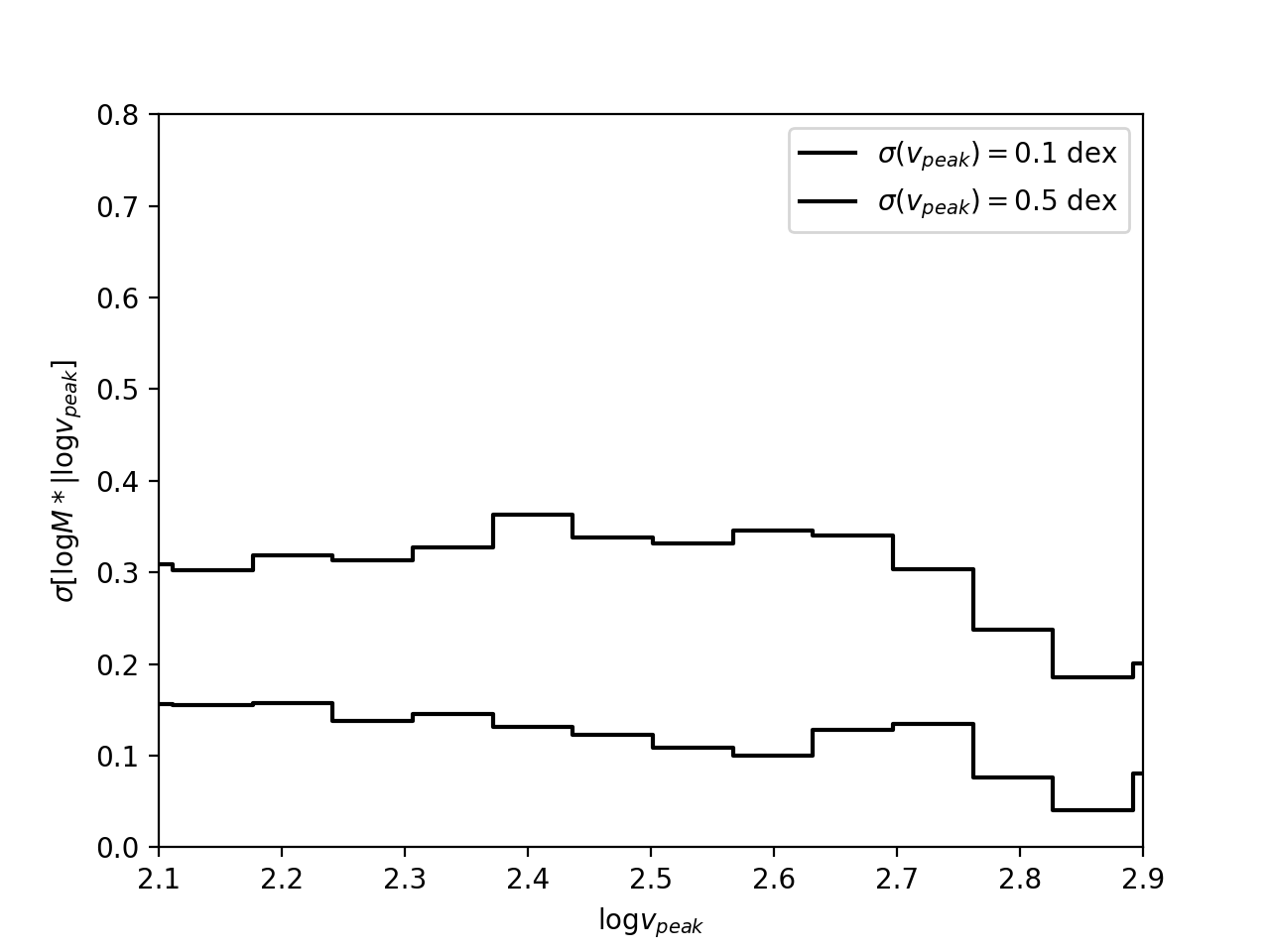
I have tried to look in more detail at the individual data points (for \(\sigma(v_{\rm peak})=0.1\) dex):
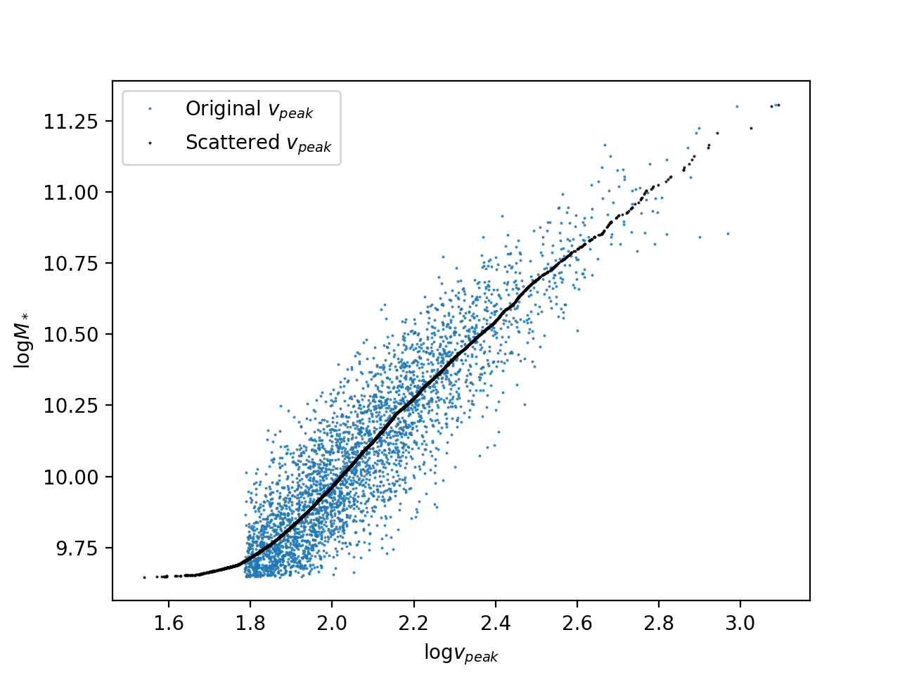
This plot shows the original data points in blue, and then the scatter that is added for the abundance matching is shown in black. This mostly looks reasonable, and the scatter in \(M_*\) agrees with the scatter I am measuring.
There is some concern that the halo mass function I am using (1) does not extend to lower \(v_{\rm peak}\) than that measured in the simulation and (2) has some problems at high \(v_{\rm peak}\) that comes from discreteness issues. This can seen by looking closer at the abundance matching (log-log plot versus the linear plot shown in the previous post):
Therefore, to fix these problems, I should use a parametric form for the halo mass function, rather than that measured directly from the simulation.
Next, I checked whether the relationship between \(M_*\) and \(v_{\rm peak}\) looks reasonable. For comparison, see the following plot from Cao et al. 2019:
The values look similar around \(\log v_{\rm peak}=2.4\). After that, mine isn’t as flat, and before that mine isn’t as steep. This could be the reason my plot for how the scatter maps does not match.
What’s Next
Use a parameterized halo mass function, see if this helps.