Nicole Drakos
Research Blog
Welcome to my Research Blog.
This is mostly meant to document what I am working on for myself, and to communicate with my colleagues. It is likely filled with errors!
This project is maintained by ndrakos
Halo Mass Function
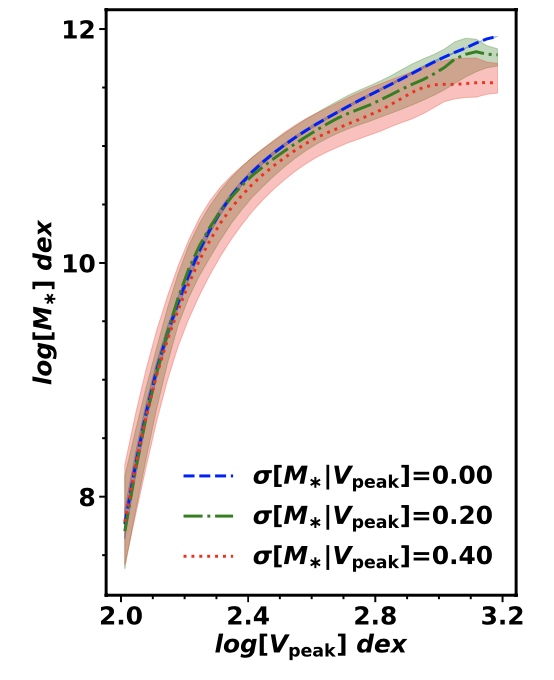
In a previous post, I realized the relation between stellar mass, \(M_*\) and \(v_{\rm peak}\) did not look right in my abundance matching results. Ideally, I would like to reproduce the following plot from Cao et al. 2019:
My \(M_*\) and \(v_{\rm peak}\) Relation
Right now, I am using the stellar mass function from Li & White 2009 and the distribution of \(v_{\rm peaks}\) measured from my sample simulation. This results in the following relation:
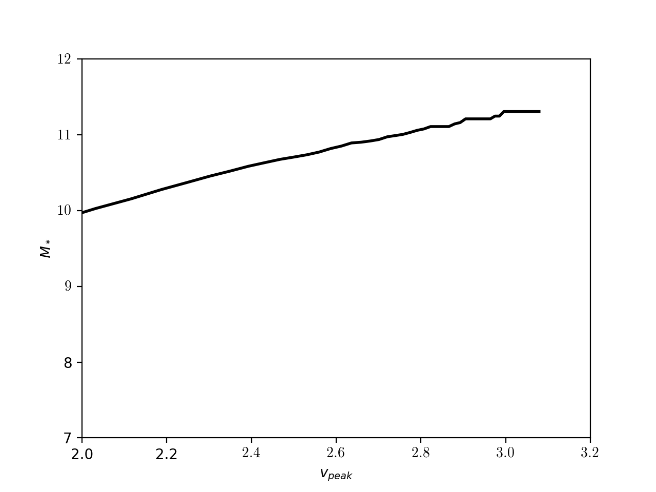
which clearly doesn’t match the plot from Cao et al. 2019.
It could be that my halo mass function is not correct (either in my calculation, or because of the resolution of the simulations). Alternatively, there could be an issue in the merger trees I am using to track \(v_{\rm peak}\). In this post, I will be testing the former.
Halo Mass Function – Theoretical
First, I will check that the halo mass function measured from the simulation agrees with theory. The halo mass function can be calculated as:
\[\dfrac{dn}{d \ln M} =f (\sigma) \dfrac{\rho_b}{M} \dfrac{d \ln \sigma^{-1}}{d \ln M}\]where \(dn/d\ln M\) is the comoving number density of halos and \(\rho_b=\Omega_M \rho_c\) is the comoving background density (with \(\rho_c = 3 H^2/8 \pi G\)), is the critical density. Note that to convert this to \(\log\) space, \({dn}/{d \log M} =\ln(10) {dn}/{d \ln M}\)
Multiplicity Function
There are many of parameterizations of the multiplicity function, \(f(\sigma)\), in the literature: I will be using the parameterization from Despali et al. 2016 , which is based off of the functional form from Sheth & Tormen 1999:
\[2 \nu f(\nu) = A \left(1 + \dfrac{1}{(a\nu)^p}\right) \left( \dfrac{2 a \nu}{\pi} \right)^{1/2} e^{-a\nu/2}\]The peak height is defined as \(\nu \equiv \delta_c^2(z)/\sigma^2(M)\). Note that \(f(\nu)d\nu = 2 \nu f(\nu) d \ln \sigma^{-1}\). The critical overdensity, \(\delta_c(z)\) is well approximated by (Kitayama & Suto 1996):
\[\delta_c(z) \approx \dfrac{3}{20} (12 \pi)^{2/3} [1 + 0.0123 \log \Omega_M (z)]\]This model has three free parameters, \((a, p, A_0)\). I am using a spherical overdensity criteria of \(200\rho_c\) (these are options in AHF); for redshift zero, this corresponds to \((a,p,A_0)=(0.903,0.322,0.287)\).
Finally, I need to calculate the fluctations, \(\sigma\).
Calculating \(\sigma (M)\)
I will make some approximations in calculating the amplitude of fluctuations, \(\sigma(M)\): this could be calculated more carefully, using the actual realization of the power spectrum, \(P(k)\), measured from the simulations (see Despali et al. 2016 ), however, for the purposes of this test, I don’t need it to be that accurate.
The fluctuations are given by:
\[\sigma^2(M,z) = \int_0^\infty P(k) W^2(kR(M)) k^2 dk\]The relationship between mass and radius is given by \(\rho_c = M/(4 \pi R^3/3)\) . \(W\) is the smoothing filter. For a top-hat filter, it is given by:
\[W (kR) = 3 \left[ \dfrac{\sin kR}{(kR)^3} - \dfrac{ \cos kR}{(kR)^2} \right]\]For the power spectrum, I will use:
\[P(k) = A k^n T^2(k)\]where \(n\) is the slope of the initial perturbation spectrum, and \(A\) is an amplitude that can be determined by setting the value of the cosmological parameter \(\sigma_8\). For the transfer function, \(T\), I will use the formula from BBKS:
\[T(k) = \dfrac{\ln (1+2.34 q)}{2.34 q}\left[1 + 3.89q + (16.1q)^2 + (5.46q)^3 + (6.71q)^4\right]^{-1/4}\]where \(q=k/\Omega_M h\) (assuming no baryon content). Note that for all these equations, \(k\) is in units of \(1/(h^{-1}Mpc)\) . I will use the following parameters: \(\Omega_M=0.3\), \(n=1\), \(\sigma^2(R = 8 h^{-1} Mpc) = 0.8^2\) and \(h=0.7\).
With this, I calculate \(\dfrac{d \ln \sigma^{-1}}{d \ln M}\) numerically.
Results
Here is the comparison between the simulation and the theoretical halo mass functions:
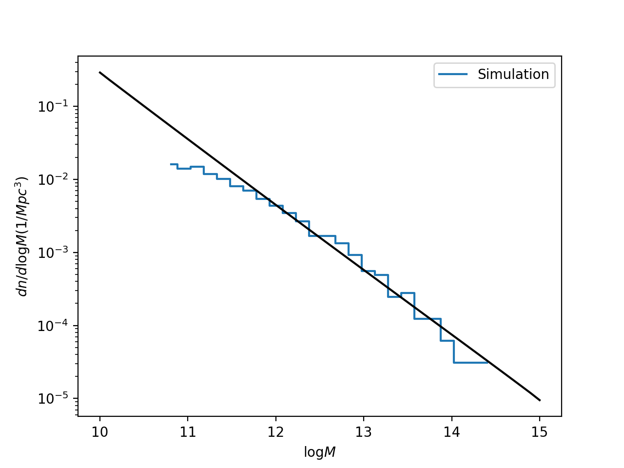
These agree pretty well above \(\log M = 12\), but I’m still not convinced I don’t have an error in my halo mass function. Either way, the steep part of the stellar to halo mass relation corresponds to masses less than that (from the \(\sigma[M \mid v_{\rm peak}]\) plot in the previous post, \(\log M=12\) corresponds roughly to \(\log v_{\rm peak} = 2.6\)). Therefore, I am pretty sure this is a resolution issue.
Update: I fixed a couple bugs in the calculation, and the halo mass function looks right now (see next post), and the conclusion it isn’t resolved seems to hold up.