SED Pipeline

As discussed in the previous post, we are changing the SED assignment method to speed up the code.

Note that this post is only concerning star-forming galaxies (SFGs). I will revisit the quiescent galaxies later.

Overview of Method

As outlined in the previous post, this method involves creating a “base” catalog that samples parameter space, and has all 7 assigned parameters (mass (\(M\)), redshift (\(z\)), metallicity (\(Z\)), gas ionization (\(U_S\)), age (\(a\)), star-formation time \(\tau\) and dust attenuation (\(\bar \tau_v\) ), as well as the resulting parameters (SFR (\(\psi\)), \(M_{UV}\) and \(\beta\)).

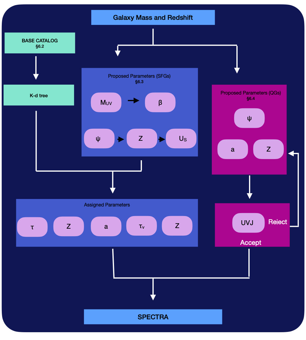
For the galaxies in the galaxy catalog (each with a fixed mass and redshift) I propose 5 parameters from known scaling relations (\(Z\), \(U_S\), \(\psi\), \(M_{UV}\) and \(\beta\)), and find closest 10 points in parameter space in base catalog and use a weighted average to assign the 5 FSPS parameters (\(Z\), \(U_S\), \(a\), \(\tau\) and \(\bar \tau_v\)). Then, FSPS is used to calculate the spectra.

Here is a rough schematic of the SED pipeline:

Base Catalog

For now I am using the 16000 galaxies from the previous post for the base catalog. This has the advantage of sampling the correct parts of parameter space. However it has very sparse sampling of low redshift galaxies, and doesn’t have that many objects. This will limit the accuracy of the method.

Test Method

I ran this method on the full \(512^3\) catalog, and found the resulting properties for the galaxy catalog:

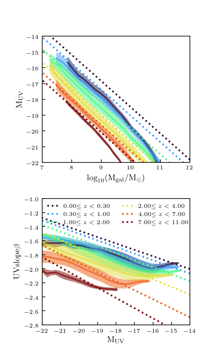
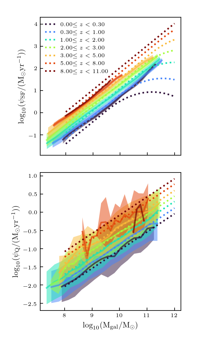
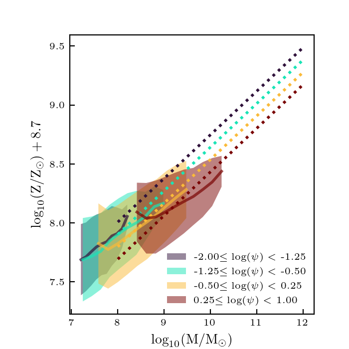
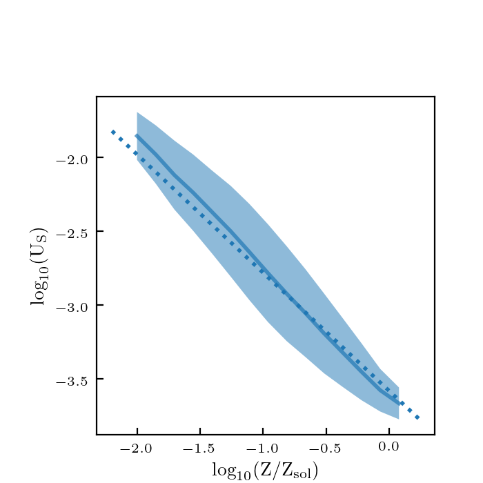
This matches the desired trends pretty well, except the UV properties at low redshifts. This is probably due to the fact that the base catalog is very sparsely sampled at low redshift. In addition, right now the distances are all effectively in different units. They should be normalized.

Better Metric

I re-ran the code with scaled parameters used to calculate the distances: \(z/12\), \(\log_{10} (M/M_\odot)/12\), \(\log_{10} (\psi/(M_\odot/ {\rm yr}))/4\), \(\log_{10}(Z/Z_\odot)/2\), \(\log_{10} U_S/4\), \(M_{\rm UV}/30\), and \(\beta/3\). Here are how the plots look now:

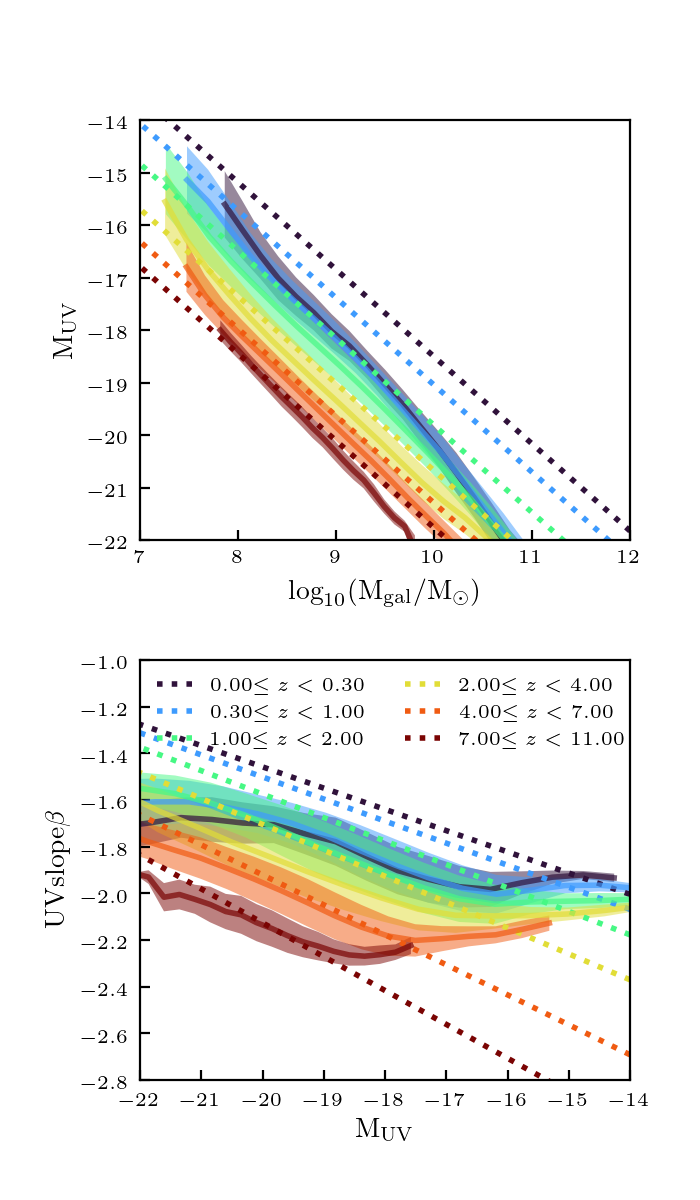
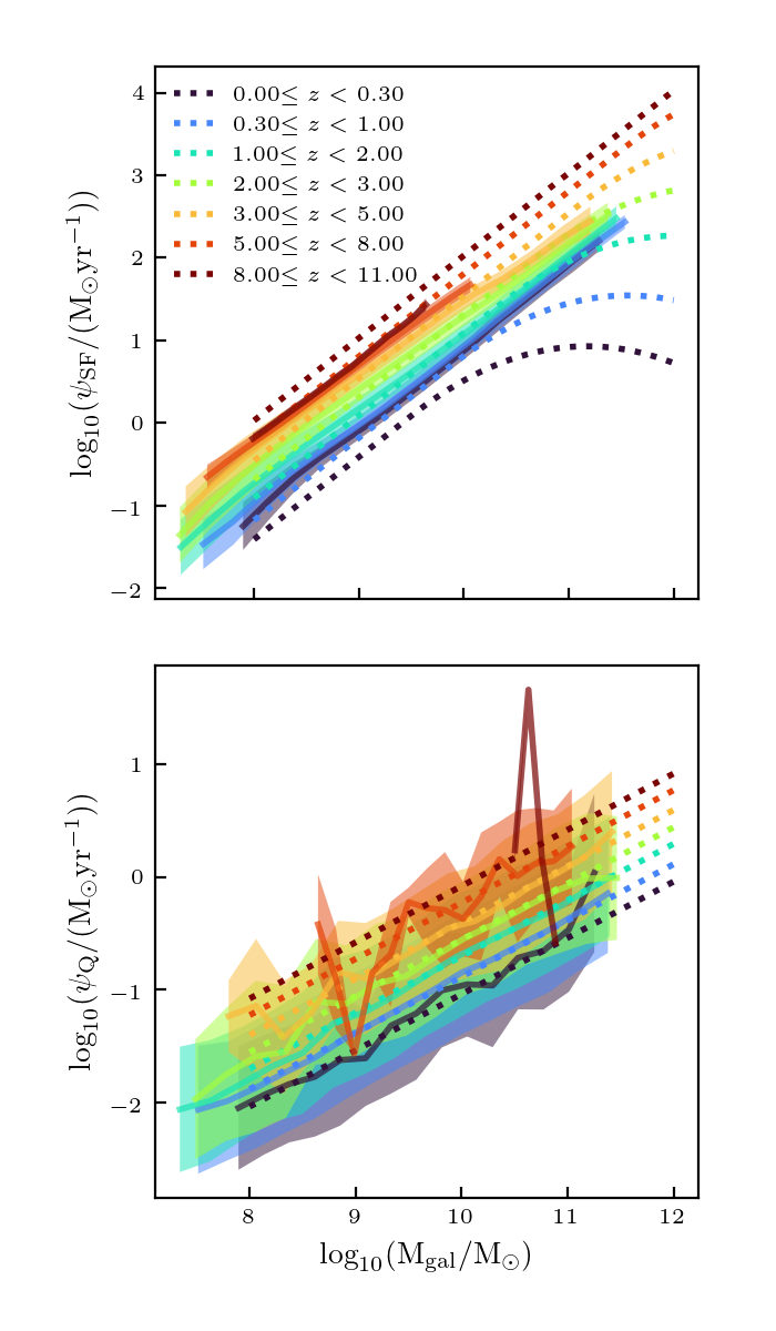
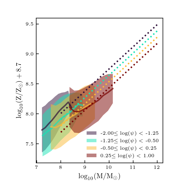
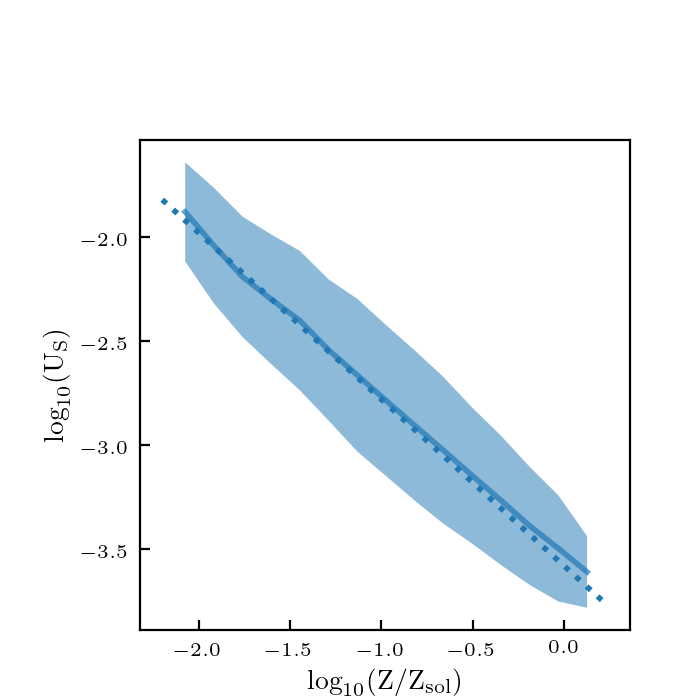
These look about the same as before, so this didn’t really make a big difference.

Timing Notes

There should be about 100x more objects in \(2048^3\) catalog (see the previous post). There are 3 steps to take in to consideration when trying to determine how fast this will be on the larger simulation:

1. Generating the base catalog

2. Generating the k-d tree

3. Generating the galaxy catalog (propose parameters, find distance on tree, generate spectra)

It took about 2.5 hours on 400 cores for the \(512^3\) catalog (which has ~\(2 \times 10^6\) objects) to finish steps 2 and 3. Right now, since the tree is small, the dominant time is generating the spectra.

Step 1: this requires 1 FSPS call per galaxy, and therefore should take about the same amount of time as this test case for the same number of objects. Therefore a base catalog of \(10^8\) is probably reasonable, and would take about 1 day to generate on 400 cores.

Step 2: I haven’t timed this yet. It was pretty much instantaneous for this base catalog (16000 galaxies).

Step 3: This step can be broken into 3 parts: (a) propose parameters: this step should be negligible compared to the other steps. (b) find the distance on tree to get new parameters. This will depend on the size of the base catalog. (c) generate spectra: generating the spectra should scale with the number of objects. I expect to take about 1 day for the \(2048^3\) simulations on 400 cores.

Plan for Updated Base Catalog

I need to find out if steps 2 and 3b are reasonable for a base catalog of size \(10^8\). If so, I can go ahead and generate a base catalog (that can be used with all the simulations).

Another thing to decide is how to sample parameter space. I want to make sure that the relevant parts of parameter space are sampled properly, but also don’t want to sample regions of parameter space that will not be populated.

My current plan is to sample uniformly in redshift and \(\log_{10} (M/M_\odot)\) over the mass and redshift range of the simulations. I will then assign \(\psi\), \(Z\) and \(U_S\) from scaling relations with scatter, to get reasonable values of metallicity and gas ionization. I will then sample age, tau and dust within reasonable ranges (see Williams et. al 2018 for reasonable distributions/ranges to use for these).

---

« Changes to SED Method

SED Pipeline Part II »