Nicole Drakos
Research Blog
Welcome to my Research Blog.
This is mostly meant to document what I am working on for myself, and to communicate with my colleagues. It is likely filled with errors!
This project is maintained by ndrakos
Two Component ICs
Here are my notes on setting up the two-component ICs that Bradley will use in his project.
IC Model
I decided to use the double power-law in Ogiya et al. 2018, as outlined here:
\[\rho(r) = \dfrac{\rho_s}{(r/r_s)^\alpha (1 + r/r_s)^{\beta - \alpha}}\]The parameters \(\alpha\) and \(\beta\) control the inner and outer slopes of the density profile, respectively. An NFW profile has (\(\alpha\), \(\beta\))=(1,3) and the Hernquist profile has (\(\alpha\), \(\beta\))=(1,4).
Truncation of Density Profile
One issue that comes up with this profile is that for certain choices of parameters, the mass profile diverges (i.e. the total mass is infinite as you go out to very large radii). In these cases, to set up the ICs you need to make some sort of truncation on the density profile.
This double power-law profil diverges if \(\beta \leq 3\). To understand this, realize the mass goes as \(\rho r^3\).. Therefore, \(\rho\) needs to drop off faster than \(r^3\). At large \(r\), \(\rho \propto r^{-\alpha} r^{-(\beta + \alpha)} \propto r^{-\beta}\).
Since \(\beta\) controls the outer slope of the satellite, it isn’t important to vary this parameter. In this post, I had planned to use \(\beta_{stars}=4\) and \(\beta_{dm}=3\). Instead, I’ll probably use \(\beta_{stars}=\beta_{dm}=4\), which should give a converging mass profile. I could also try \(\beta_{dm}=3.1\), if I decide I want the dark matter component to be more extended. This really shouldn’t effect the results much though.
The “Alpha” Profile
I am going to set \(\beta=4\), and call the following the “alpha” profile (for lack of a better name):
\[\rho(r) = \dfrac{\rho_s}{(r/r_s)^\alpha (1 + r/r_s)^{4 - \alpha}}\]In the Alpha profile, \(\alpha\) sets the inner slope, \(r_s\) sets the scale radius, and \(\rho_s\) sets the total mass.
Here is the profile, varying \(\alpha\):

Mass Profile
To set-up the desired ICs, need to know the relation between \(\rho_s\) and mass:
\[M(<r) = \int_0^r \rho(r') 4 \pi r'^2 dr'\] \[M(<r) = \dfrac{4 \pi \rho_s r_s^3 }{3-\alpha} \left[ \dfrac{r}{r_s+r}\right]^{3-\alpha}\]And the total mass is:
\[M = \dfrac{4 \pi \rho_s r_s^3 }{3-\alpha}\]Gravitational Potential
\(\Delta \phi = 4 \pi G \rho(r)\), with boundary conditions \(d\phi/dr(0)=0\) and \(\phi(r \rightarrow \infty)=0\)
\[\dfrac{1}{r^2}\dfrac{d}{dr}\left( r^2 \dfrac{d\phi}{dr} \right) = 4 \pi G \rho(r)\] \[\phi = - \dfrac{4 \pi G \rho_s r_s^2}{(3-\alpha)(2-\alpha)} \left[ 1 - \left(\dfrac{x}{x+1}\right)^{2-\alpha} \right]\]And the central potential is
\(\phi_0 = -\dfrac{4 \pi G \rho_s r_s^2}{(3-\alpha)(2-\alpha)}\).
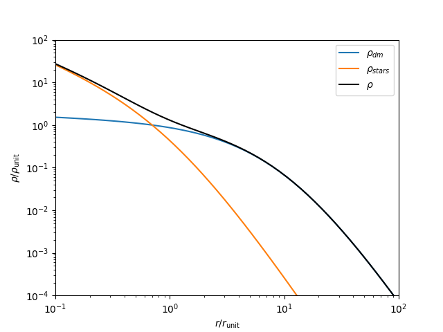
Fiducial Profile
For the “fiducial” profile, I had decided
- \(\alpha_{dm}\) = 0.1
- \(\alpha_{stars}\) = 1
- \(r_{s,dm}/r_{s,stars}\) = 10
- \(M_{dm}/M_{stars}\) = 200
which looks like this:
I will primarily change the alpha values of both components, but maybe also explore different size and mass ratios. I will also mostly stick to one set of orbital parameters to start (next post on this topic…).
Calculating the Distribution Function
As outlined here, the distribution function can be calculated as:
\[f_i(\mathcal{E})=\dfrac{1}{\sqrt{8}\pi^2}\left[ \int_{r_{\mathcal{E}}}^\infty \dfrac{1}{\sqrt{\mathcal{E}- \Psi}}\dfrac{d^2 \rho_i}{d \Psi^2} \dfrac{GM}{r^2} dr \right]\] \[\dfrac{d^2 \rho_i}{d \Psi^2} = \left( \dfrac{r^4}{G^2 M^2} \right) \left[ \dfrac{d^2 \rho_i}{d r^2} + \left( \dfrac{r^2}{GM} \right) \left[\dfrac{2GM}{r^3} -4\pi G\rho\right] \dfrac{d \rho_i}{d r} \right]\]I got this working on a Double Hernquist profile previously.
For the Alpha model (where \(p=\rho/\rho_s\), \(x=r/r_s\) ):
\[\dfrac{dp}{d x} = - \dfrac{p (\alpha + 4x)}{x(1+x)}\] \[\dfrac{d^2 p}{d x^2} = \dfrac{p }{x^2(1+x)^2} (\alpha^2 + 20 x^2 + 10 x\alpha + \alpha)\]Given all this, I can add this to my IC code, ICICLE.